How do labs train a frontier, multi-billion parameter model? We look towards Hugging Face’s SmolLM3, Prime Intellect’s Intellect 3, Nous Research’s Hermes 4, OpenAI’s gpt-oss-120b, Moonshot’s Kimi K2, and DeepSeek’s DeepSeek-R1. This blog is an attempt at distilling the techniques, motivations, and considerations used to train their models with an emphasis on training methodology over infrastructure.

These notes are largely structured based on Hugging Face’s SmolLM3 report due to its extensiveness, and it is currently supplemented with notes from other reports including Intellect-3, gpt-oss-120b, Hermes 4, DeepSeek, and Kimi. Also, these notes have not been thoroughly reviewed. Any errors are entirely my responsibility.

While this blog explores some infrastructure-related ideas like in-flight weight updates and multi-client orchestrators, there are many other ideas mentioned throughout those posts/blogs like expert parallelism and quantization. Hugging Face writes more about gpt-oss-120b’s infrastructure here.

general practices

“Learn to identify what’s worth testing, not just how to run tests. Perfect ablations on irrelevant choices waste as much compute as sloppy ablations on important ones.”
- Ablations need to be fast (faster iteration $\rightarrow$ more hypotheses tested) and reliable (need strong discriminative power because otherwise, it may be noise)
- “The real value of a solid ablation setup goes beyond just building a good model. When things inevitably go wrong during our main training run (and they will, no matter how much we prepare), we want to be confident in every decision we made and quickly identify which components weren’t properly tested and could be causing the issues. This preparation saves debugging time and keeps our sanity intact. There’s nothing worse than staring at a mysterious training failure with no idea where the bug could be hiding.”
Choose an established baseline with good architecture and training setup design. These take years of iteration, and people have discovered common failure modes and instabilities.
- There are a plethora of modifiable components (attention mechanisms and positional encodings to name a few), but follow the principle of derisking: “never change anything unless you’ve tested that it helps.”
In evals, look for monotonicity (score improvement), low noise (e.g. score resistance to random seeds), above-random performance (random-level performance for extended time frames isn’t useful), and ranking consistency (ranking of approaches should remain stable throughout training).
- Prioritize evals! Between pre-training and post-training, core evals should be preserved, and their implementation should be finished long before the base model is finished training.
Balance exploration and execution. For methods, choose flexibility and stability over peak performance, set a deadline for exploration.

architecture and set-up

Architecture decisions fundamentally determine a model’s efficiency, capabilities, and training dynamics. Model families like DeepSeek, gpt-oss-120b, Kimi, and SmolLM have vastly different architectures (dense vs MoE), attention mechanisms (MHA vs MLA vs GQA), position encodings (RoPE, partial RoPE, NoPE), among many others. Not all information about the models is publicly available, so some are chosen:

	Kimi-K2	gpt-oss-120b	OLMo 3	SmolLM
Parameter Count	1.06T	116.83B	32B	3B
Attention	MLA	GQA (8 groups)	GQA (?)	GQA (4 groups)
Positional Embedding	RoPE (?) + YARN	RoPE + YARN	RoPE + YARN	RNoPE + YARN
Architecture	MoE	MoE	dense	dense
Tokenizer	tokenization_kimi	o200k_harmony	cl_100k	Llama3

When choosing architecture, Hugging Face suggests following a decision tree such that if one of these is true, choose a dense architecture:

memory-constrained (since MoEs must have all experts loaded)
new to LLM training (focus on basics)
tighter timeline (simpler training with well-documented recipes)

attention

Multi-head attention (MHA) uses separate query, key, and value projections for each attention head, but this creates a large KV-cache that becomes an inference bottleneck and GPU memory hoarder. To address this, researchers developed multi-query attention (MQA) and grouped query attention (GQA). In MQA, KV values are shared across all heads, but this comes at a cost of leaking attention capacity because heads can’t store information specialized to each head’s role. GQA softens this issue by sharing KV values across a small group of heads (e.g. 4). Another alternative is multi-latent attention (MLA) which stores a compressed latent variable that can be decompressed/projected into KV values at runtime. The latent variable is typically much smaller than the full KV cache (often achieving 4-8x compression), and this results in a KV-cache parameter count more comparable to GQA while maintaining performance stronger than MQA.

When ablating (for variables that change the parameter count such as changing MHA to GQA, they occasionally adjust other hyperparameters to keep model sizes roughly the same), Hugging Face found that GQA with small groups beats MHA and that MHA beats MQA and GQA with 16 groups. Across benchmarks like HellaSwag, MMLU, and ARC, GQA with 2/4/8 groups does best.

document masking

When pre-training, a common consideration is fixed sequence lengths since training uses tensors of the form [batch, sequence length, hidden], so with regards to batching and distributed training, GPUs are most happy when every example has the same sequence length. But due to variable document length and wanting to avoid padding which wastes compute, packing enables shuffling and concatenating documents within the same sequence to achieve the sequence length.

Causal masking means that for unrelated files $A$ and $B$ in the same batch, the tokens in $B$ can attend to the tokens in $A$, which degrades performance. With intra-document masking, the attention mask is modified so tokens can only attend to previous tokens within the same document. Many papers have found benefits relating to long-context extension and some short context benchmarks as well as shortening the average context length.

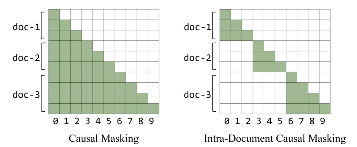
Comparison of causal masking vs intra-document masking showing attention patterns

Figure 1: Comparison of causal masking (left) and intra-document masking (right). Causal masking allows tokens to attend to all preceding tokens regardless of document boundaries, while intra-document masking restricts attention to tokens within the same document. From @PMinervini.

When implementing document masking, Hugging Face saw small improvements on PIQA but otherwise no noticeable impact on short context tasks. But in line with aforementioned research, they observed that it became crucial for scaling from 4k to 64k tokens.

Input embeddings (token-to-vector lookup) and output embeddings (hidden states to vocab logits) are typically represented as separate matrices, so the total embedding parameters are $2 \times \text{vocab size} \times \text{hidden dim}$. In small language models, this can account for up to 20% of total parameters, as is the case with Llama 3.2 1B (in larger models, the embeddings represent a much smaller fraction of the parameter count, only 3% in Llama 3.1 70B). The issue with tying them is that input/output embeddings still represent different geometries, and frequent tokens like “the” can dominate representation learning due to getting gradients from both the input stream and the predicted output.

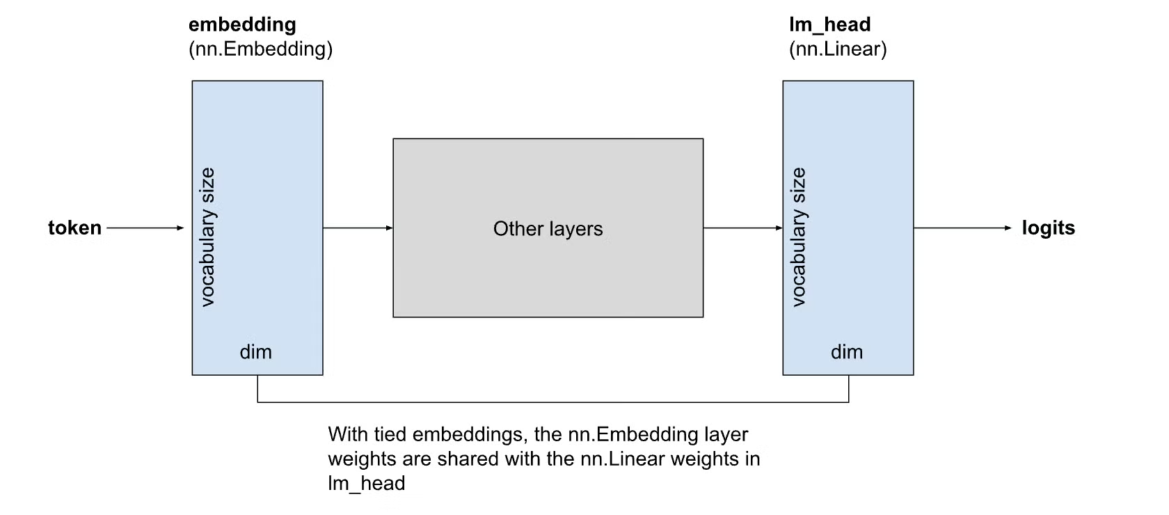
Comparison of tied vs untied embedding architectures

Figure 2: Comparison of untied embeddings (separate input and output matrices) vs tied embeddings (shared matrix). Tied embeddings reduce parameter count while maintaining comparable performance. From PyTorch Blog.

Hugging Face found that on a 1.2B model, tied embeddings did comparably well despite having 18% fewer parameters (down from 1.46B), and that compared to an untied model also with 1.2B parameters (fewer layers), untied showed higher loss and lower downstream eval scores.

positional encodings

Without positional encoding, transformers have no sense of word order, akin to the bag of words idea. Initially, absolute position embeddings were used by learning a lookup table that mapped the position index to a vector added to token embeddings, but the maximum input sequence length was limited by the sequence length it was trained on. Relative position encodings followed since capturing distance between tokens matters more than capturing their absolute positions.

The most commonly used technique is rotary position embedding (RoPE), which encodes position information by rotating query and key vectors in 2D planes. RoPE encodes relative position as rotation angles: based on the dimensionality of the query/key vector, RoPE splits it into pairs (since they rotate in 2D space) and rotates depending on the absolute position of a token and a base frequency. During attention, the dot product between their rotated positions directly encodes their relative distance via the phase difference in their rotation angles, where tokens $x$ positions apart always maintain the same angular relationship.

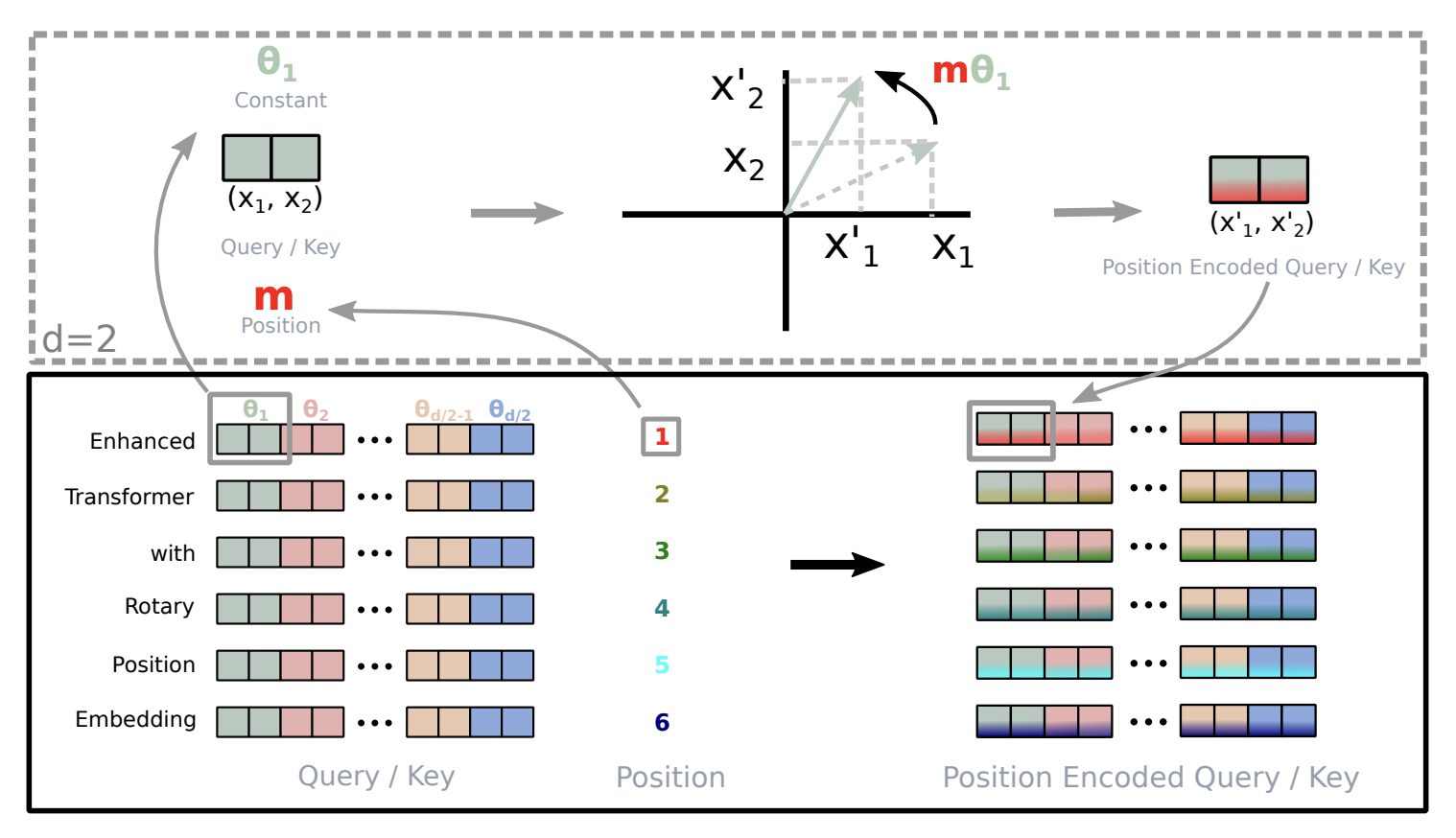
RoPE positional encoding showing rotation of query/key pairs in 2D space

Figure 3: RoPE splits query/key vectors into pairs and rotates each pair by an angle proportional to position. From Su et al., 2021.

During pre-training, models are trained on shorter context lengths (similar ideas to document masking, and quadratic attention is expensive) to learn short range correlation between words. But as sequence length grows, the rotation angles grow via $\theta= \text{position} \times \frac1{\text{base}^{\frac{k}{\text{dim}/2}}}$. This can be fixed by increasing the base frequency as the sequence length increases using methods like ABF (Adaptive Base Frequency) or YaRN, which applies a more granular interpolation of frequencies on different components and includes other techniques like dynamic attention scaling and temperature adjustment. For extremely long contexts, YaRN does best, and in gpt-oss-120b, it was used to extend the context length of dense layers up to 131k tokens.

More recently, with the emphasis on long contexts, NoPE (no position embedding) and RNoPE, a hybrid method, have emerged. NoPE uses only causal masking and attention patterns, so it doesn’t bump into the issue of extrapolating beyond training lengths but shows weaker performance on short context reasoning and knowledge-based tasks. RNoPE alternates applying RoPE and NoPE on attention blocks, where RoPE handles local context and NoPE helps with longer-range information retrieval. Another idea is Partial RoPE, which applies RoPE/NoPE within the same layer.

Hugging Face ran ablations using RoPE, RNoPE (removing positional encoding every 4th layer), and RNoPE with document masking. They found that all achieve similar performance on short-context tasks, so they adopt RNoPE + document masking because it provides the foundation for long-context handling.

attention for long contexts

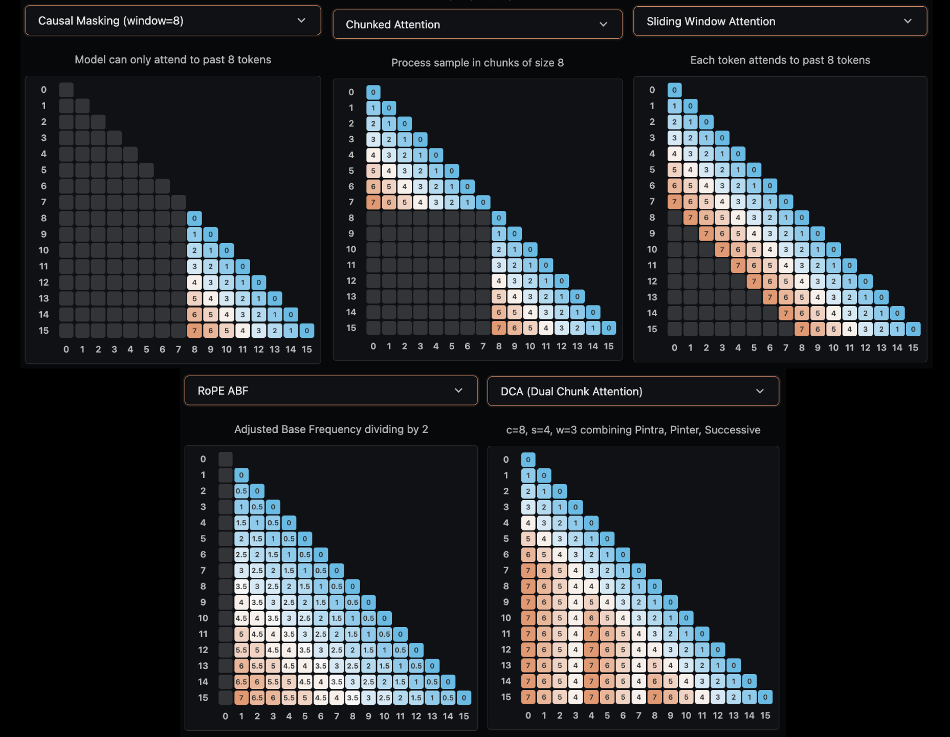Attention patterns comparison showing causal masking, chunked attention, sliding window attention, RoPE ABF, and DCA Figure 4: five common types of attention. From Hugging Face.

An alternative to adjusting positional encodings for long contexts is specifying the strength with which tokens can attend to one another.

Chunked Attention: divides the sequence into fixed-sized chunks where tokens can only attend within their chunk. Llama 4 pairs RNoPE (specifically the RoPE layers) which also reduces the KV cache size per layer, but its performance on long context tasks degraded.
Sliding Window Attention (SWA): every token can see up to $p$ positions back, creating a sliding window that maintains local context. Gemma 3 combined SWA with full attention every other layer.
Dual Chunk Attention (DCA): $K$ tokens are chunked into $M$ groups. Within each group (like chunked attention), tokens attend normally. Between successive chunks, there is a local window to preserve locality, and more broadly, inter-chunk attention allows queries to attend to previous chunks with a capped relative position cap. Qwen-2.5 used DCA to support context windows of up to 1 million tokens.

MoE

MoEs (mixture of experts), analogous to our brain activating different regions for different tasks, provide an alternative to dense models. At inference, only certain “experts” are activated based on the input, dramatically reducing compute compared to dense models where all parameters are active. The MoE works by replacing the feed forward layer with multiple MLPs (experts) and adding a learnable router before the MLPs to select the experts. The router typically uses top-k gating, selecting the $k$ experts with highest affinity scores for each token, where $k$ is usually much smaller than the total number of experts (e.g., 8 out of 384).

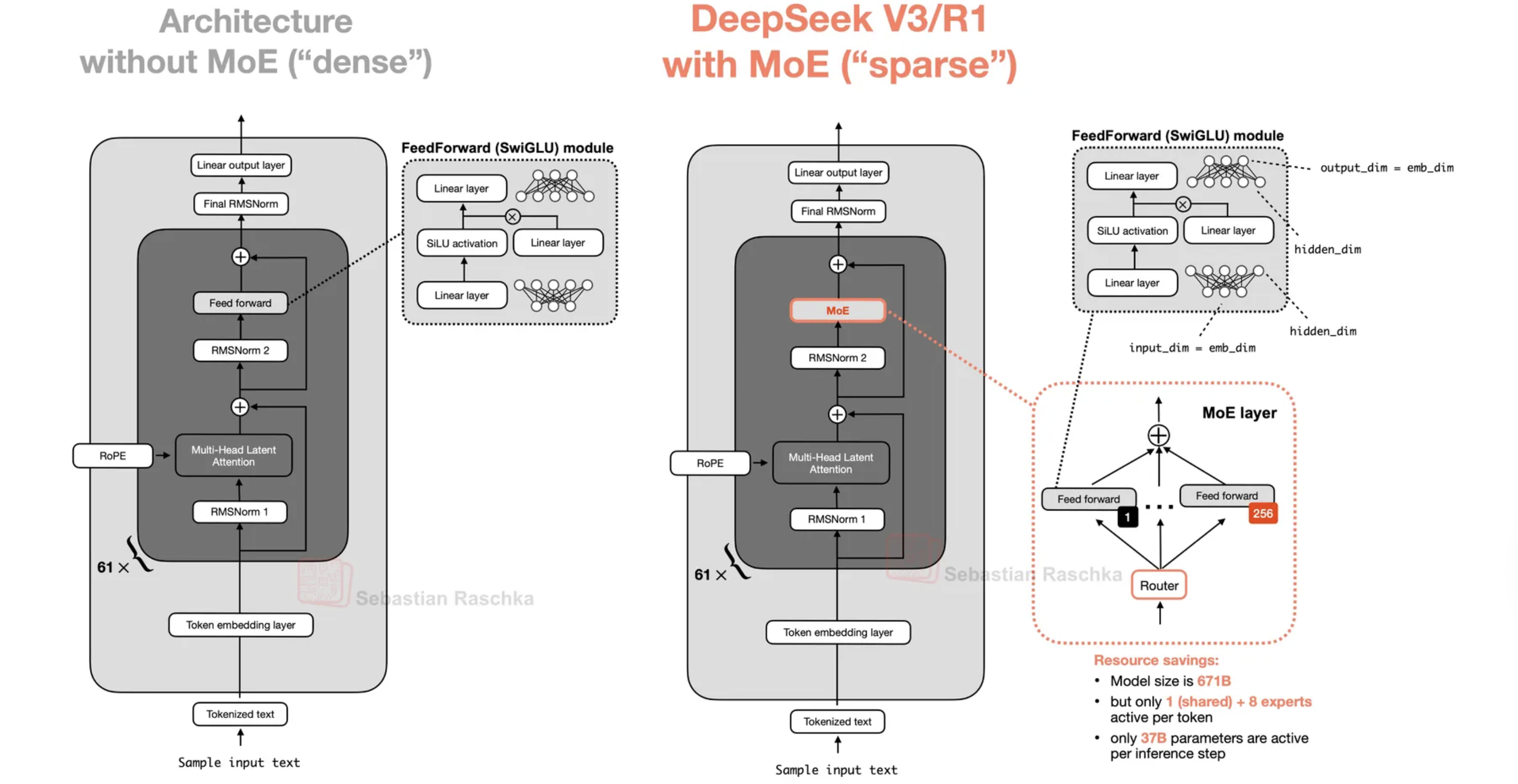Figure 5: Comparison of dense architecture and MoE architecture. From Sebastian Raschka.

In general, for fixed number and size of active experts, increasing the total number of experts improves loss, and high sparsity improves performance and benefits more from increasing compute. Recent models are much more sparse, with over 100 experts and around 10 active per token.

To determine how large each expert should be, a common metric is granularity, defined by $G = 2 \cdot \frac{d_\text{model}}{d_\text{expert}}$, where a higher granularity corresponds to more experts with a smaller dimension; this can be interpreted as a number proportional to the experts needed to match the dense MLP width. Recent models have granularity anywhere from 2 (gpt-oss-120b) to 8 (qwen3-next-80b-a3b). Ant Group showed that granularity doesn’t significantly change loss but does drive efficiency leverage (the ratio of flops needed for an MoE to achieve the same loss as a dense model). And overall, MoEs present a good alternative to dense models in terms of compute for training and inference.

Shared experts are always-on experts, which absorb the basic, recurring patterns so that other experts can more aggressively specialize; one is often enough (DeepSeek-V2 uses two, which adds a bit of complexity).

Load balancing is crucial in that if it fails, not only do training and inference efficiency plummet, but so do effective learning capacity. The routing mechanism typically uses top-k gating: for each token, the router computes affinity scores (often via a learned linear projection followed by softmax), selects the top $k$ experts, and routes the token to those experts. To ensure balanced expert utilization, this can be addressed by adding a loss-based load balancer (LBL) given by $\mathcal{L} = \alpha \sum_{i=1}^{N_r} f_i P_i$ where $\alpha$ determines the strength, $f_i$ is the fraction of tokens going through expert $i$, and $P_i$ is the probability mass that sums the probability of tokens going through an expert; so in perfect load balancing, $f_i=P_i=\frac1{N_r}$. Also, $\alpha$ should not be so large that routing uniformity overwhelms the primary training objective. These should be monitored using global statistics, not local statistics which may suffer from a local batch being narrow, biasing the routing statistics.

DeepSeek-V3 does loss-free load balancing differently, by adding a bias term to affinity scores going into the routing softmax.

hybrid models

Because transformers don’t deal efficiently with long context while RNNs can, one idea is to combine both to get the best of both worlds. By dropping the softmax from the output for token $t$:

\[\mathbf{o}_t = \sum_{j=1}^t \frac{\exp(\mathbf{q}_t^\top \mathbf{k}_j)\mathbf{v}_j}{\sum_{l=1}^t \exp(\mathbf{q}_t^\top \mathbf{k}_l)} \Longrightarrow \mathbf{o}_t = \sum_{j=1}^t (\mathbf{q}_t^\top \mathbf{k}_j)\mathbf{v}_j = \left(\sum_{j=1}^t \mathbf{v}_j \mathbf{k}_j^\top\right)\mathbf{q}_t\]

And by defining $S_t :=\sum_{j=1}^t \mathbf{k}_j \mathbf{v}_j^\top$, then we get a recurrent relation where $S_t$ summarizes all past $(k_j, v_j)$.

\[S_t=S_{t-1}+\mathbf{k}_t \mathbf{v}_t^\top \Longrightarrow \mathbf{o}_t = S_t \mathbf{q}_t = S_{t-1}\mathbf{q}_t+\mathbf{v}_t\left(\mathbf{k}_t^\top \mathbf{q}_t\right)\]

While this gets us closer to an RNN-esque structure, in practice, softmax stabilizes training, and the linear form can cause instability without normalization. With RNNs, it is sometimes helpful to forget the past, by introducing a gate $\mathbf{G}_t$ for the previous state $\mathbf{S}_t=\mathbf{G}_t \odot \mathbf{S}_{t-1} + \mathbf{v}_t\mathbf{k}_t^\top$ Mamba-2 is among the most popular, being used in hybrid models like Nemotron-H and Falcon H1. Hybrid models are becoming increasingly popular, notably in Qwen3-Next with a gated DeltaNet update and Kimi’s next model, likely using their “kimi delta attention.”

stability

Training stability is crucial for successful large-scale model training. Several techniques help prevent training failures, including regularization methods, careful initialization, and architectural choices. The following sections cover key stability mechanisms:

$z$-loss

$z$-loss is a regularization term added to the standard cross entropy loss that keeps logits from drifting to large magnitudes. The softmax denominator is $Z = \sum_{i=1}^V e^{z_i}$, and by adding $\mathcal{L} = \lambda \cdot \log^2(Z)$ to the loss, we penalize based on $\log(Z)$ which represents the overall logit scale.

On their 1B model, Hugging Face found that adding $Z$-loss didn’t impact training loss or downstream performance, so they chose not to include it due to training overhead.

removing weight decay from embeddings

Despite being a regularization technique, removing weight decay from embeddings can improve training stability. Weight decay causes embedding norm to decrease, but this can lead to larger gradients in earlier layers since the LayerNorm Jacobian has a $\frac1{\sigma}$ term (coming from normalization) which is inversely proportional to the input norm $\sigma$.

Hugging Face tested this using a weight decay baseline, a no weight decay baseline, and another combining all previous adopted changes and found no significant loss or eval results, so they included no weight decay.

qk norm

Similar to $z$-loss, QK-norm helps prevent attention logits from becoming too large by applying LayerNorm to both the query and key vectors before computing attention. However, the same paper which proposed RNoPE found that it hurts long-context tasks because the normalization demphasizes relevant tokens and emphasizes irrelevant tokens by stripping the query-key dot product of its magnitude.

other design considerations

Parameter initialization: either normalization initialization ($\mu=0$, $\sigma=0.02, 0.006$) with clipping (often with $\pm 2-3 \sigma$) or a scheme like $\mu\text{P}$ (maximal update parametrization) which dictates how weights and learning rates should scale with width so that training dynamics stay comparable.
Activation Function: SwiGLU is what most modern LLMs use, not ReLU or GeLU; for example, gpt-oss-120b uses gated SwiGLU. Some exceptions are Gemma2 using GeGLU and nvidia using $\text{relu}^2$.
Width vs Height: deeper models tend to outperform equally sized wider ones on language modeling and compositional tasks. In smaller models, this is more pronounced, but larger models make use of wider models for faster inference due to modern architectures supporting better parallelism.

tokenizer

There are a few considerations that typically guide tokenizer design:

domains: in domains like math and code, digits and other special characters require careful treatment. Most tokenizers do single-digit splitting, which helps with arithmetic patterns more effectively and prevents memorization of numbers. Some tokenizers like Llama3 further encode numbers 1 to 999 as unique tokens.
supported languages: a tokenizer trained on english text would be extremely inefficient if it encountered another language, say mandarin or farsi.
target data mixture: when training a tokenizer from scratch, we should train on samples that mirror our final training mixture.

Larger vocabularies can compress text more efficiently, but they come at the cost of a larger embedding matrix, which as mentioned in the embeddings section, can take up a sizable portion of the parameter count. For english-only models, 50k is often enough, while multilingual models need over 100k. There is an optimal size that exists since compression gains from larger vocabularies decrease exponentially.

Large models benefit from large vocabularies since the extra compression saves more on the forward pass (project to QKV, attention, and MLP) than the additional embedding tokens during softmax. For memory, larger vocab means fewer tokens, so a smaller KV cache.

BPE (byte-pair encoding) still remains the de facto choice. Starting with tiny units (e.g. characters or bytes), the BPE algorithm repeatedly merges the most common adjacent pair into a new token. To evaluate a tokenizer’s performance, fertility is a common metric, measuring the average number of tokens needed to encode a word (alternatively, characters-to-tokens ratio or bytes-to-tokens ratio, but these have limitations due to word length variability and byte representations). Another is proportion of continued words, describing what percentage of words get split into multiple pieces. For both, smaller metrics indicate more efficient tokenizers.

There are many strong existing tokenizers, like GPT4’s tokenizer and Gemma3’s tokenizer. Often, using existing tokenizers is enough; only when we want to train for low-resource languages or have a different data mixture should we continue training our own tokenizer.

optimizers and training hyperparameters

Choosing optimizers and tuning hyperparameters is notoriously time-consuming and significantly impacts convergence speed and training stability. While we may be tempted to distill those from models of larger labs (albeit a useful prior), it may not fit the use case.

adamW

Despite being invented over 10 years ago, AdamW still stands the test of time. Adam (adaptive momentum estimation) updates weights individually based on an exponential weighted average of gradients $g_t$ and an exponential weighted average of squared gradients $g_t^2$, along with weight decay (the “W”). The exponential moving averages provide adaptive learning rates per parameter: parameters with consistently large gradients get smaller effective learning rates (via the squared gradient term), while parameters with small or noisy gradients get larger effective learning rates. This adaptivity helps stabilize training and converge faster:

\[\begin{align*} \theta &\leftarrow (1-\alpha \lambda)\theta - \alpha \frac{\hat{m}_t}{\sqrt{v_t}+\epsilon} \\ \hat{m}_t &= \frac{m_t}{1-\beta_1^t}, \quad m_t = \beta_1 m_{t-1} + (1-\beta_1) g_t \\ \hat{v}_t &= \frac{v_t}{1-\beta_2^t}, \quad v_t = \beta_2 v_{t-1} + (1-\beta_2) g_t^2 \end{align*}\]

Even for modern LLMs, the hyperparameters remain largely unchanged: weight decay factor $\lambda=0.1$ or $\lambda=0.01$, $\beta_1=0.9$, and $\beta_2=0.95$.

muon

Unlike AdamW which updates per-parameter, muon treats the weight matrix as a singular object and updates based on matrix-level operations. This approach reduces axis-aligned bias (where optimization favors certain coordinate directions) and encourages exploration of directions that would otherwise be suppressed. By considering the entire weight matrix structure rather than individual parameters, muon can better capture correlations between parameters:

\[\begin{align*} g_t &\leftarrow \nabla_\theta \mathcal{L}_t(\theta_{t-1}) \\ B_t &\leftarrow \mu B_{t-1} + G_t \\ O_t &\leftarrow \text{NewtonSchulz5}(B_t) \\ \theta_t &\leftarrow \theta_{t-1} - \eta O_t \end{align*}\]

where $B_0=0$, and NewtonSchulz5 describes the odd function $f(x)=3.4445x-4.7750x^3+2.0315x^5$. This blog and this blog describe the algebra of it in more detail as well as why the coefficients are what they are. The Newton-Schulz iteration approximates the matrix sign function: we can estimate the SVD decompositions of $G=U \Sigma V^\top$ by $UV^\top$, and $f(x)$ essentially replaces $\Sigma$ because iteratively applying $f$ (i.e., $f \circ f \circ \cdots f(x)$) converges to the sign function, which normalizes the singular values. This has the effect of reducing axis-aligned bias and encouraging exploration of directions that would otherwise be suppressed. Also, muon can tolerate higher batch sizes.

But since muon operates at the matrix level, applying NewtonSchulz requires access to the full gradient tensor. One method uses an overlapping round-robin scheme where each rank is responsible for gathering all gradient matrices corresponding to its index and applying muon locally. Since FSDP expects sharded gradients/updates, and every rank has its shard of the muon-updated gradient, then the optimizer step can proceed normally. However, this issues lots of overlapping collectives across many matrices which breaks at scale.

The alternative that Prime adapts is based on all-to-all collectives which does bulk permutation so that each rank temporarily owns full gradients for its matrices, runs muon, then bulk permutes them back. This may require padding since many tensors are packed into contiguous buffers which can change the size that’s expected. However, this requires fewer collectives and scales better.

Building on Muon, Kimi K2 introduces MuonClip, a stabilization technique that prevents exploding attention logits, which is a common failure mode in large-scale training. Other strategies include logit soft-cap, which applies $\tanh$ clipping to the pre-softmax logits, or QK norm, which applies LayerNorm to the QK matrices. However, these lead to issues of the scaled dot-product exploding (making bounding too late) and distorted gradients around regions where the model is unstable in logit soft-cap, and key matrices are not materialized during inference (projected from a latent variable).

For each attention head $h$, consider $\mathbf{Q}^h$, $\mathbf{K}^h$, and $\mathbf{V}^h$. For a batch $B$ and input representation $\mathbf{X}$, define the max logit as a per-head scalar to be the maximum input to softmax

\[S_\text{max}^h = \frac1{\sqrt{d}} \max_{\mathbf{X} \in B} \max_{i, j} \mathbf{Q}_i^h \mathbf{K}_j^{h\top}\]

Set $S_\text{max} = \max_h S_\text{max}^h$ and target threshold $\tau$. The idea is to rescale $\mathbf{W}k$ and $\mathbf{W}_q$ whenever $S\text{max}^h$ exceeds $\tau$. Also, $\gamma=\min(1, \frac{\tau}{S_\text{max}})$, one approach is to clip all heads simultaneously by

\[\mathbf{W}_q^h \leftarrow \gamma^\alpha \mathbf{W}_q^h \quad \mathbf{W}_k^h \leftarrow \gamma^{1-\alpha} \mathbf{W}_k^h\]

where the $\gamma$ exponentials enforce multiplicative weight decay for $\mathbf{Q}^h \mathbf{K}^{h\top}$; commonly, $\alpha=0.5$ to ensure equal scaling to queries and keys. However, not all heads exhibit exploding logits, which motivates a per-head clipping based on $\gamma_h = \min(1, \frac{\tau}{S_\text{max}^h})$, which is more straightforward for MHA but less for MLA. The challenge with MLA is that keys are projected from a latent variable rather than materialized directly, so clipping must be applied to the latent-to-key projection weights and the latent variable itself. They apply clipping only on $\mathbf{q}^C$ and $\mathbf{k}^C$ (head-specific components) scaled by $\sqrt{\gamma_h}$, $\mathbf{q}^R$ (head-specific rotary) scaled by $\gamma_h$, and $\mathbf{Q}^R$ (shared rotary). Besides that, the main muon algorithm is modified to match Adam RMS and enable weight decay. For each weight $\mathbf{W} \in \mathbb{R}^{n \times m}$:

\[\begin{align*} g_t &\leftarrow \nabla_\theta \mathcal{L}_t(\theta_{t-1}) \\ B_t &\leftarrow \mu B_{t-1} + G_t \\ O_t &\leftarrow \text{NewtonSchulz5}(B_t) \cdot \sqrt{\max(n,m)} \cdot 0.2 \\ \theta_t &\leftarrow (1-\eta \lambda)\theta_{t-1} - \eta O_t \end{align*}\]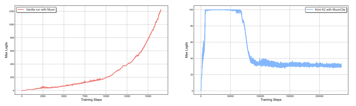

Figure 6: Left: a mid-scale training run on a 9B active, 53B total MoE where attention logits diverge quickly. Right: maximum logits for KimiK2 with MuonClip and $\tau=100$, where max logits eventually decays to a stable range after ~30% of the training steps. From Kimi K2.

learning rates

Learning rates have their own life cycle: they warmup (typically 1%-5% of training steps for short trainings, but large labs fix the warmup steps) from zero to avoid chaos, then anneal after settling into a good minimum. Cosine annealing was the go-to scheduler, but it’s also inflexible due to the cosine period needing to match the total training duration. Alternatives include warmup-stable-decay (WSD) and multi-step; in the last x% of tokens, the former linearly decays the learning rate whereas multi-step does discrete drops. For WSD, typically 10-20% is allocated for the decay phase, matching cosine annealing; in multi-step, 80/10/10 also matches cosine annealing while 70/15/15 and 60/20/20 can outperform it. Deepseek-v3 used cosine annealing between the decay drops and added a constant phase before the final sharp step.

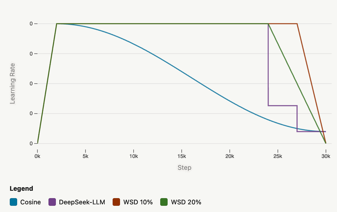Learning rate schedules comparison Figure 7: Comparison of learning rate schedules: cosine annealing, WSD, and multi-step. From Hugging Face.

Hugging Face’s ablations (on their 1B model) showed that WSD tended to underperform cosine annealing before WSD’s decay began, but once it entered its decay phase, WSD showed nearly linear improvement in both loss and eval metrics, which allowed it to catch up to cosine annealing by the end. After running further ablations on the learning rate, the Hugging Face team settled on 2e-4; increasing led to potential increased risk of instability during long training runs. Kimi K2 also uses WSD: the first 10T were trained with 2e-4 learning rate after a 500 step warm up, then 5.5T tokens with cosine decay from 2e-4 to 2e-5.

WSD schedule especially helps with ablations since it does not require restarting the same run for different token counts, since we can retrain only the end portions (learning rate decay) while maintaining the front portion.

batch size

There is a critical batch size: too small and we may be underutilizing compute, but too large and the model needs more tokens to reach the same loss. Still, larger batch sizes give more efficient gradient estimations, and are preferred.

A useful proxy is that for optimizers like AdamW or Muon, if the batch size increases by a factor of $k$ then the learning rate should scale up by $\sqrt{k}$. Intuitively, larger batches provide more stable gradient estimates (lower variance), so we can afford larger step sizes. Mathematically, the covariance shrinks by a factor of $k$, and based on the SGD parameter update $\Delta w = -\eta g_B$, we have $\text{Var}(\Delta w) \sim \eta^2 \frac{\Sigma}{B}$ where $B$ is the original batch size. To maintain the same update variance, we need $\eta \sim \sqrt{k}$.

As training progresses, the critical batch size grows. Initially, since the model is making large updates, $\lvert \lvert g \rvert \rvert^2$ is large so the model should have a small critical batch size. After the model stabilizes, larger batches become more effective. This motivates the idea of batch size warmup.

scaling laws

Scaling laws (e.g. Chinchilla scaling laws) provide a useful proxy for determining how aggressively/conservatively to update hyperparameters as model size scales.

First, $C \approx 6 \cdot N \cdot D$ where $C$ is the compute budget measured in FLOPs, N is the number of parameters, and $D$ is the number of training tokens. The 6 is derived from empirical estimates for the number of FLOPs per parameter.

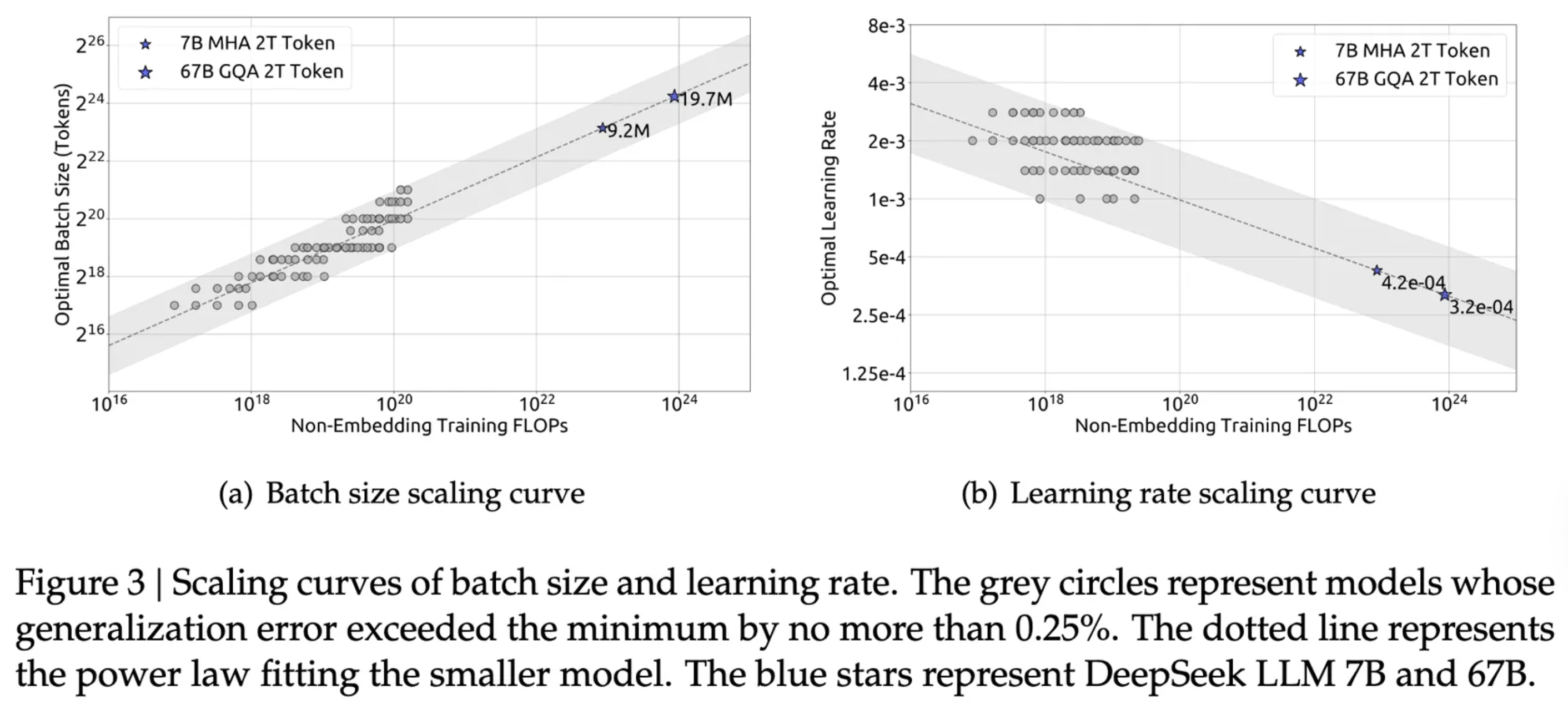Figure 8: Scaling curves of batch size and learning rate. From DeepSeek.

Initially, scaling laws indicated that language model size was the main constraint, leading to a GPT-3 model with 175B parameters but only trained on 300B tokens. A re-derivation found that training duration could improve gains more than size; they found that compute-optimal training of GPT-3 should have consumed 3.7T tokens.

However, scaling laws are almost never religiously followed. Recently, labs have been “overtraining” models beyond the training durations suggested by scaling laws (e.g. Qwen 3 being trained on 36T tokens). Moreover, “compute-optimal” scaling laws don’t account for larger models being more expensive after training due to inference. To that end, Hugging Face decided to train on 11T tokens on a 3B model. For comparison, Kimi K2’s 1T model comprised of 15.5T pre-training tokens.

While general scaling laws provide guidance, Kimi K2’s scaling law analysis revealed model-specific insights. They showed that an increase in sparsity, the ratio of total number of experts to the number of activated experts, yields substantial performance improvements for fixed FLOPs, so they increase the number of MoE experts to 384 (256 in DeepSeek-V3) while decreasing attention heads to 64 (128 in DeepSeek-V3) to reduce computational overhead during inference. They settle on a sparsity of 48, activating 8 out of 384 experts and found that decreasing the attention heads from 128 to 64 sacrificed a validation loss ranging from 0.5% to 1.2%, but a 45% decrease in inference FLOPs.

data curation and pre-training

Even with the perfect architecture, a model’s performance is still heavily dependent on its training data; no amount of compute or optimization can compensate for training on the wrong content. To this end, it’s about assembling the right data mixture, balancing training objectives and tuning data proportions. This is particularly difficult since across competing objectives, for a fixed compute budget, increasing one proportion necessarily decreases another, hurting performance.

There already exist large corpora of pre-training datasets like FineWeb2 and The Pile. However, there are still a plethora of information gaps, so recent models additionally rely on specialized pretraining datasets for domains like math and coding.

One consideration is data quality. Of course, training on the highest quality data possible is preferable. But for a training budget of $X$ tokens, because high quality data is limited, only filtering for it would lead to repeated data, which can be harmful. So, an ideal mixture includes both higher and lower quality data.

Another consideration is model safety. For gpt-oss-120b, OpenAI addresses this by filtering the data for harmful content in pre-training, with an emphasis on hazardous biosecurity knowledge. They use CBRN (chemical, biological, radiological, and nuclear) pre-training filters that were used in GPT-4o.

multi-stage training

Multi-stage training, the idea of evolving the data mixture as training progresses, can better maximize both high-quality and lower-quality data compared to a static mixture because a LM’s final behavior is heavily dictated by the data it sees at the end of training. So, this motivates the strategy of saving the higher quality data towards the end. This introduces another variable of when to begin changing mixtures, and a general principle to performance-driven intervention: if a benchmark begins to plateau, it’s a signal to introduce high-quality data for that domain.

ablation

While architectural ablations are done on smaller models (e.g. on 1B models to train for 3B models), data mixture ablations are done at scale because larger models have much larger capacities to understand a variety of domains. Moreover, annealing ablations are done on checkpoints of the main run (like 7T out of 11T tokens) to determine what datasets to introduce when.

To determine optimal data proportions, recent models often use a validation loss or a holdout loss to minimize based on evaluation objectives and data domains. However, some of these methods tend to converge toward distributions that mirror the dataset size distribution, and they don’t outperform careful manual ablations.

token utility

Token efficiency is how much performance improvement is achieved per token consumed during training. This can be improved via better token utility, the effective learning signal each token contributes; this motivates finding the optimal balance of high-quality tokens, since they should be maximally leveraged but also limited to prevent overfitting and reduced generalization.

Kimi K2 uses data rephrasing in knowledge and math domains. For knowledge, this comes in the form of style and perspective-diverse prompting to rephrase the texts, chunk-wise autoregressive generation to gradually build a rephrased version of long documents, and fidelity verification to ensure semantic alignment. In the main training run, each corpus is rephrased at most twice. For math, diversity is increased via rephrasing into a “learning-note style” and translation into other languages.

pre-training data

SmolLM3

Hugging Face’s goal was to build a multi-lingual model that also excels on math and coding. In stage 1 of their multi-stage training, they use a 75/12/10/3 split among english web data, multilingual web data, code data, and math data.

English web data: they ablate on a mixture of FineWeb-Edu (educational and STEM benchmarks) and DCLM (common sense reasoning), two strong open English web datasets at the time of training, finding that a 60/40 or a 50/50 split was best. Later, they add in other datasets including Pes2o, Wikipedia & Wikibooks, and StackExchange.
Multilingual web data: five European languages were chosen, with data from FineWeb2-HQ. Smaller portions of other languages, like Chinese or Arabic, were chosen to allow others to do continual pretraining of SmolLM3. Ultimately, they found that 12% multilingual content in the web mix was best.
Code data: primarily extracted from The Stack v2 and StarCoder2, it includes 16 languages, Github PRs, Jupyter/Kaggle notebooks, Github issues, and StackExchange threads. Despite research showing that code improves LM performance beyond coding, they did not observe this effect (rather a degradation on English benchmarks) using the recommended code mixture. They delay adding their educationally filtered subset, Stack-Edu, following the principle of delaying the best data until the end.
Math data: using FineMath3+, InfiWebMath3+, MegaMath, and instruction/reasoning datasets like OpenMathInstruct and OpenMathReasoning.

For new stages (using a checkpoint at around 7T out of the total 11T tokens), they use a 40/60 split between the baseline mixture and the new dataset. SmolLM3 has three stages: 8T tokens @ 4k context for base training, 2T tokens @ 4k context for high-quality injection, and 1.1T tokens @4k context a reasoning/Q&A stage.

hermes 4

Using data from DCLM and FineWeb, Nous first performs semantic deduplication using embeddings at a cosine similarity of 0.7, and then uses an LLM-as-judge to filter out incomplete or ill-formatted messages. Then, they process pre-training data through DataForge, a graph-based synthetic data generator, which allows for large and complex structures. By taking a random walk through a directed acyclic graph where nodes implement a mapping from struct $\to$ struct such that if there is an edge from node $A$ to node $B$, the postconditions guaranteed by $A$ must satisfy the preconditions of $B$. QA pairs are generated using this workflow with intermediary transformations into other mediums (e.g. a wikipedia article into a rap song), question generation and then questions/answers annotations using an LLM-as-judge to grade the instruction and response. Also, to find a covering set of data-scarce domains of special interest, they recursively (depth-first-search) generate a taxonomy of subdomains where the leaves are prompts and the LLM enumerates $n$ subdomains to form a partition.

The DataForge-generated data is used in both pre-training and post-training stages, with specific details provided in the post-training data section below.

mid-training

Mid-training is the intermediary step between pre-training and post-training where the base model is trained further on a large amount of domain-specific tokens, especially shaping the model to focus on common core skills like coding or reasoning. Often-times, the decision to mid-train is only made after initial SFT experiments are run because they may reveal performance gaps that indicate the need to mid-train on certain domains. But if the goal is to elicit shallow capabilities like style or conversation, the compute is better spent in post-training.

Some recipes include an additional long context stage; for example, Qwen3 first trained on 30T tokens at 4k context, then a reasoning stage with 5T higher-quality tokens mainly on STEM and coding, and finally a long context stage at 32k context length.

SmolLM3 also does this, but instead of scaling from 4k to 128k directly, they sequentially scale from 4k to 32k to 64k to 128k, which allows the model to adapt at each length before pushing the context length further. Upsampling long context documents like web articles or books improve long context, but Hugging Face didn’t observe improvement; they hypothesize that this is because their baseline mixture already includes long documents using RNoPE.

To go from 4k to 32k and later to 64k, they use RoPE ABF and increase the base frequency to 2M and 5M, respectively. Base frequencies like 10M further improved slightly on RULER, long context benchmark, but it hurt short context tasks like GSM8k, so they were disregarded. To reach 128k, they found that using YARN from the 64k checkpoint (instead of using a four-fold increase from 32k) produced better performance, which confirms the hypothesis that training closer to the desired inference length benefits performance.

Kimi K2 decays learning rate from 2e-5 to 7e-6, training on 400B tokens with 4k sequence length, then 60B tokens with a 32k sequence length. To extend to 128k, they use YARN.

While the mid-training data usually comes from web data, another powerful approach is to use distilled reasoning tokens from a better model, as Phi-4-Mini-Reasoning did from DeepSeek-R1. When applied to the base model, distilled mid-training increased benchmark scores like AIM24 by 3x, MATH-500 by 11 points, and GPQA-D by almost 6 points. SmolLM3 also does distilled mid-training. They considered datasets including reasoning tokens from DeepSeek-R1 (4M samples) and QwQ-32B (1.2M samples) but decide to delay using the Mixture of Thoughts dataset until the final SFT mix. They found that it almost always makes sense to perform some amount of mid-training if the base model hasn’t already seen lots of reasoning data during pre-training, because they noticed that /no_think reasoning mode also had improvements on reasoning benchmarks.

post-training

evals

Given today’s standards of LLMs as coding agents and assistants that can reason, there are four broad classes of evals that researchers care about:

Knowledge: for small models, GPQA Diamond tests graduate-level multi-choice questions and gives better signal than other evals like MMLU. Another good test for factuality is SimpleQA, although smaller models are much less performant due to limited knowledge.
Math: AIME is still the leading benchmark, with others like MATH-500 providing a useful sanity check for small models.
Code: LiveCodeBench tracks both coding competency via competitive programming while SWE-bench Verified is a more sophisticated alternative but much harder for smaller models.
Multilinguality: there aren’t many options except for Global MMLU to target the languages that models were pretrained on/should perform well in.

These evals test the following:

Long context: RULER, HELMET, and more recently-released MRCR and GraphWalks benchmark long-context understanding.
Instruction following: IFEval uses verifiers against verifiable instructions, and IFBench extends upon it with a more diverse set of constraints. For multi-turn, Multi-IF and MultiChallenge are preferred.
Alignment: LMArena with human annotators and public leaderboards is the most popular. But due to the cost of these evaluations, LLM-as-judge evals have emerged, including AlpacaEval and MixEval.
Tool calling: TAU-Bench tests a model’s ability to use tools to resolve user problems in customer service settings, including retail and airline.

To prevent overfitting, evals that encapsulate robustness or adaptability, like GSMPlus which perturbs problems from GSM8k, are also included. Another way is using interval evals or vibe evaluations/arenas, such as manually probing the model’s behavior. Other tips include using small subsets to accelerate evals (especially if there’s correlation with a larger eval), fixing the LLM-as-judge model (if the eval requires it), treat anything used during ablations as validation, use avg@k accuracy, and try not to (don’t) benchmax!

post-training data

intellect 3

It’s first worth mentioning that Intellect-3 is a 106B parameter MoE (12B activate) post-trained on top of GLM-4.5-Air base model from Z.ai, and that they have their own post-training stack including prime-rl, an open framework for large-scale asynchronous RL, verifiers library for training and evals from their Environments Hub, sandbox code execution and compute orchestration.

Integrating with the Environments Hub, Prime trains on a diverse and challenging mix of environments designed to improve coding and reasoning capabilities. For math, they design an environment with long CoT reasoning in mind, consisting of 21.2K challenging math problems from Skywork-OR1, Acereason-Math, DAPO, and ORZ-Hard, all of which are curated datasets derived from AIME, NuminaMath, Tulu3 math, and others which test difficult math questions from multiple choice to proofs to those involving figures. Even using verifiers, there were a non-trivial amount of false negatives, so they additionally use opencompass/CompassVerifier-7B as a LLM-judge verifier. For science (mainly physics, chemistry, and biology), they filter 29.3K challenging problems from MegaScience while also using LLM-judge verification and standard math verifiers. For logic (games like Sudoku or Minesweeper), 11.6K problems and verifiers were adapted from SynLogic.

For code, they primarily use their Synthetic-2 dataset along with Prime Sandboxes to verify solutions. They also develop two SWE environments that support scaffolding for common formats like R2E-Gym, SWE-smith, and Multi-SWE-bench to fix issues within a Github project when equipped to Bash commands and edit tooling. Also, the maximum number of turns for the agent is set at 200.

Prime also focuses on its deep research capabilities via their web search environment, which provides the model with a set of search tools. The environment tasks the model with answering questions from the dataset using tools and is rewarded either 1 or 0 using z-AI’s DeepDive dataset, with 1K samples for SFT trajectory generation and 2.2K samples for RL. When tested in Qwen/Qwen3-4B-Instruct-2507, 26 steps of SFT with batch size of 34 followed by 120 steps of RL at a group size of 16 and batch size of 512 was enough to reach mean reward of 0.7.

hermes 4

They use 300k prompts, mostly STEM and coding from WebInstruct-Verified, rSTAR-Coder, and DeepMath-103k and apply deduplicating and filtering for prompts with >2k characters.

Nous rejection samples against ~1k task-specific verifiers using Atropos. Some environments used to generate the dataset include

Answer Format Training: rewards succinctly-presented final answers, like $\mathtt{\backslash boxed{}}$ in LaTeX, but there are over 150 output formats sampled. The environment also enforces <think> and </think> delimiters.
Instruction Following: leverages RLVR-IFEval for sets of verifiable tasks with constraint instructions like “Every $n^\text{th}$ word of your response must be in French.”
Schema Adherence: facilitates generation (producing a valid JSON object from natural language prompt and a schema) and editing (identifying and correcting validation errors within a malformed JSON object)
Tool Use: facilitates agentic behavior by training the model to generate reasoning and produce tool calls via the <tool_call> token.

kimi k2

A critical capability that Kimi K2 chooses to focus on is tool use. While benchmarks like $\tau$-bench and ACEBench exist, it’s often difficult to construct real-world environments at scale due to cost, complexity, privacy, and accessibility. Kimi K2 builds off of ACEBench’s data synthesis framework to simulate real-world tool-use scenarios at scale:

Tool spec generation: constructing a large repo of tool specs from real-world tools and LLM-synthetic tools
Agent and task generation: for each tool-set sampled from the repo, generate an agent to use the toolset on some corresponding tasks
Trajectory generation: for each agent/task, generate trajectories where the agent finishes the task

Using 3k+ real MCP tools from Github and 20k synthetic tools generated hierarchically in domains like financial trading, software applications, and robot control. Diversification among agents is ensured via the combination of distinct system prompts with distinct tool combinations, and tasks are graded using an explicit rubric with an LLM judge.

For RL, Kimi K2’s treatment for math, STEM, and logical tasks remains similar to those of other models. Coding and software engineering comes largely from competition-level programming problems and PRs/issues from GitHub. For instruction following, they use two verification mechanisms: deterministic evaluation via code interpreters for verifiable outputs and LLM-as-judge evaluations for non-verifiable outputs. The data was constructed using expert-crafted prompts and rubrics, agentic instruction augmentation inspired by AutoIF, and a fine-tuned model specialized for generating additional instructions probing specific failure modes or edge cases.

chat template

A few important considerations for designing/picking a good chat template include system role customizability, tool calling, reasoning, and compatibility with inference engines like vLLM or SGLang. Qwen3 and GPT-OSS satisfy all criteria, and Qwen3 is designed for hybrid reasoning.

In SmolLM3, despite also being designed for hybrid reasoning, they discard the reasoning content for all but the final turn in the conversation to avoid blowing up the context during inference, but for training, it’s important to retain the reasoning tokens to condition the model properly. So, Hugging Face orchestrates their own chat template, satisfying all criteria. Vibe tests initially revealed a bug of not passing in the custom instructions into their custom template, but this was quickly patched.

While deriving inspiration from the Qwen3 template, Intellect-3 always reasons (not hybrid) by proxy of being dominantly trained on reasoning-only SFT traces; they use qwen3_coder tool call parser and deepseek_r1 reasoning parser to ensure reasoning chains are consistently represented.

gpt-oss-120b uses the harmony chat template, which introduces “channels” that determine the visibility of each message. For example, final for answers shown to the user, commentary for tool calling, and analysis for CoT tokens. This allows the model to interleave tool calls with CoT.

Hermes 4 adapts Llama 3’s chat template by changing the assistant to a first-person identifier after identifying the sensitivity to the token used for the assistant’s turn:

\[\mathtt{<\lvert start\_header\_id\rvert>assistant<\lvert end\_header\_id\rvert>} \longrightarrow \mathtt{<\lvert start\_header\_id\rvert>me<\lvert end\_header\_id\rvert>}\]

This results in markedly different behaviors, which is explored more in “behaviors and latent capabilities” subsection of “behaviors and safety” section.

DeepSeek-R1-Zero’s chat template looks very similar to others, but additionally includes $\mathtt{}$ tags to provide the final answer.

sft

Most post-training pipelines start with supervised fine-tuning (SFT) because it’s cheap compared to RL, stable due to insensitivity to reward design and hyperparameters, and gives a strong baseline off of the base model. Usually, base models are too unrefined to benefit from more advanced post-training methods. SFT often comes in the form of distillation from stronger models. Strong models may suffer from success and skip the SFT stage because there are no stronger models to distill from (such is the case with DeepSeek R1-Zero).

Dataset curation for SFT is important; datasets might seem great on paper, but models trained on those datasets may end up overindexing on certain domains, such as science. To this end, Hugging Face curated a data mixture with ~100k examples and 76.1M tokens, mostly consisting of instruction following, reasoning, and steerability for both think and non-think modes. Importantly, data should be paired across modes because otherwise, there is not an indication of when to give a concise answer or use extended reasoning.

For training, there are other considerations as well: full finetuning vs more parameter efficient methods like LoRA or QLoRA, specialized kernels like FlashAttention (which reduces memory usage by recomputing attention on-the-fly during the backward pass, trading compute for memory) or the likes of SonicMoE for more efficient compute usage, masking the loss for only assistant tokens, the type of parallelism needed, learning rate tuning, and sequence length tuning to match the distribution of data to speed up training (more useful for larger datasets).

In Intellect-3, Prime splits SFT into two stages: general reasoning SFT and agentic SFT. In the first, they use datasets consisting of math, code, science, tooling, chat, and instruction splits from Nemotron’s post-training dataset and AM-DeepSeek-R1-0528-Distilled for a total of 9.9B tokens. In the second stage, they target agentic behavior, tool use, and long-horizon control (gpt-oss-120b also targets agentic behavior and tool use), using a mix of open-source agentic datasets like SWE-Swiss and synthetically-generate datasets from the Environments Hub using DeepSeek-R1. Besides serving the purpose of fine-tuning for agentic behavior, this stage also has the effect of pushing the model toward longer effective context lengths. Using context parallelism, they scaled from a 65K context window to 98K.

In Hermes 4, they also do two stages of SFT, both around reasoning. They noted that despite training on sequences at most 16k tokens in length, the reasoning lengths frequently exceed 41k tokens on reasoning tasks. So, they do a second stage to teach the model to generate the closing $\mathtt{</think>}$ tags at 30k tokens, their budget. This insertion at a fixed token count allows the model to learn a counting behavior (“when you reach $N$ tokens, stop”) while ensuring that the model’s own distribution doesn’t change significantly. This also avoids the problem of model collapse when recursive training on full, self-generated outputs leads to distribution narrowing and quality degradation.

capabilities

The Hugging Face team found issues in generalising single-turn reasoning data to multi-turn data, stemming from the difficulty in differentiating /think and /no_think tags between turns. So, they constructed a new dataset, IFThink, using Qwen3-32B that augmented single-turn instructions into multi-turn exchanges with verifiable instructions and reasoning traces; this dramatically improved multi-turn reasoning.

Masking user turns is another design choice, since otherwise loss is computed on user queries as well, sacrificing producing high-quality assistant responses for predicting user queries. In practice, masking doesn’t have a huge impact on downstream evals, but still yielded improvements by a few points in most cases.

sequence packing

Sequence packing is another choice that improves training efficiency. The idea is similar to intra-document masking where sequences are packed into a batch so as to not waste padding compute via excessive padding tokens, but with the additional constraint of minimizing truncation of documents across batch boundaries.

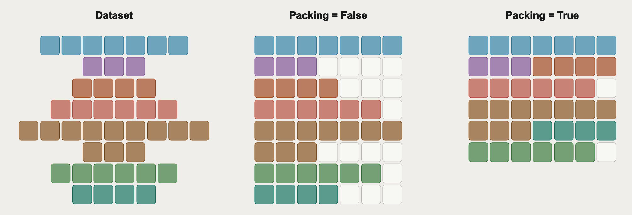Sequence packing comparison Figure 9: Comparison of sequence packing strategies. From Hugging Face.

In the image, the last packing method uses the best-fit decreasing (implemented in TRL), where each sequence is placed in the batch that minimizes the remaining space after insertion. Another method, which Hermes-4 uses, is first-fit decreasing, which places a sequence in the first batch that has enough remaining space, which achieves $>99.9\%$ batch efficiency.

Despite yielding up to a 33x tokens/batch/optimization step, for a fixed token budget, packing alters training dynamics since the more data means fewer gradient updates. This especially hurts small datasets where each sample matters more. An effective batch size of 128 hurt evals like IFEval by up to 10%; for effective batch sizes larger than 32, there was an average drop in performance (for SmolLM3 and the dataset). But for large datasets, packing is almost always beneficial.

learning rate and epochs

The learning rate for SFT is usually an order of magnitude smaller than that for pre-training since the model has already learned rich representations, and aggressive updates can lead to catastrophic forgetting. And because SFT runtime is so short compared to pre-training, it makes sense to do full learning rate sweeps. For SmolLM3, learning rates of 3e-6 or 1e-5 worked best. When packing is enabled, it’s safer to decrease the learning rate further due to the larger effective batch size and getting fewer updates for the same token budget.

Once a good data mixture is identified and hyperparameters are tuned, training on more than one epoch (what was usually done in ablations) also leads to increased performance by a few percentage points; on LiveCodeBench v4, performance nearly doubled from epoch two to three.

An interesting idea explored is whether the optimizers for pre/post-training should be the same. AdamW remains the default choice for both pre/post-training, and when tested with Muon, using the same optimiser still yielded the best performance.

preference optimization (PO)

Because SFT is fundamentally a form of imitation learning, extremely large SFT datasets can be redundant due to diminishing gains or failure modes that aren’t encapsulated in the data. Another useful signal is preference, i.e. which response, A or B, is preferred and enables model performance to scale beyond the limits of SFT alone. Also, less data is needed for preference optimization than SFT since the starting point is already strong.

For generating preference datasets, there are a few methods:

Strong vs weak: for fixed prompts $x$, strong model $S$ and weak model $W$, always prefer the stronger model’s output $y_S$ over the weaker model’s output $y_W$. This is easy to construct since the stronger model’s output is reliably better. With methods like DPO, the difference between strong and weak responses can be enforced.
On-policy with grading: using the same model and prompt, generate multiple candidate responses and have an external model (e.g. LLM-as-judges) that score responses using rubrics or verifiers that provides preference labels. This requires a well-calibrated and reliable LLM-as-judge, but also allows for ongoing bootstrapping of preference data.

While preference optimization is generally thought as a medium to improve helpfulness or alignment, it can also teach models to reason better, like using strong-vs-weak preferences.

There are typically three hyperparameters that affect training dynamics:

Learning rate: when tested across sizes of being 2x to 200x smaller than the learning rate used in SFT, Zephyr7B found that using a 10x smaller lr provided best performance improvement, and SmolLM3 ended using a 20x smaller lr (1e-6) to balance performance between /think and /no_think modes.
$\beta$: ranging from 0 to 1, it controls whether to stay closer to the reference model (loss $\beta$) or closer to the preference data (higher $\beta$). If too large, it could erase capabilities from the SFT checkpoint, so $\beta$ values around 0.1 or higher are usually preferable
preference dataset size: when tested with sizes from 2k to 340k pairs, performance largely remained stable, although Hugging Face noted performance drops in extended thinking for datasets beyond 100k pairs. To that point, don’t be afraid to create your own preference data, especially with how cheap inference has become.

algorithms

Besides vanilla DPO (direct preference optimization), researchers have explored a variety of alternatives:

KTO (Kahneman-Tversky Optimization): instead of pairs, KTO assigns updates based on whether a sample is labeled desirable/undesirable, taking ideas from human decision making along with a reference point $z_0$ and a reward-like log-ratio term.
ORPO (odds ratio preference optimization): incorporates PO with SFT via an integrated odds ratio term to the cross-entropy loss. This makes it more computationally efficient since there is no need to use a separate reference model that is used in DPO to compute $r_\theta(x,y)$.
APO (anchored preference optimization): rather than just optimizing the difference between $y^+$ and $y^-$ in DPO, APO-zero forces $y^+$ up and $y^-$ down while APO-down pushes both $y^+, y^-$ down (useful if the quality of $y^+$ is below that of the current model)

Hugging Face found that APO-zero had the best overall out-of-domain performance.

RL

SFT and PO can hit ceilings because fundamentally, they optimize to produce outputs that look like the dataset and PO is often off-policy and weak at multi-step credit assignment. RL (reinforcement learning) helps by providing a reward signal through interaction with an environment. Verifiers can automatically check correctness and provide those reward signals, and objectives can be optimized for beyond preference labels.

In RLHF (RL from human feedback), human comparisons are provided, and a reward model is trained to predict the human preference signal. Then, the policy is fine-tuned with RL to maximize the learned reward. This way, RLHF does on-policy optimization since it does rollouts using the current policy used in training and updates based on the reward given by the reward model. This also allows RLHF to discover behaviors not present in the preference dataset.

In RLVR (RL with verifiable rewards), popularised by DeepSeek-R1, verifiers check whether a model’s output matches criteria (e.g. whether it produced the correct math answer or passed all code unit tests). Then, the policy is fine-tuned to produce more verifiably-correct outputs. While RLHF requires human preference labels, RLVR uses automated verifiers (e.g., code test suites, math solvers) for reward signals, making it more scalable and objective.

Although policy optimization algorithms are commonly on-policy, like GRPO, in practice, to maximize throughput, they may actually be slightly off-policy. For example, in GRPO, without freezing the policy, generating multiple rollout batches and doing optimizer updates sequentially makes only the first batch on-policy and all subsequent batches off-policy; this is known as in-flight updates.

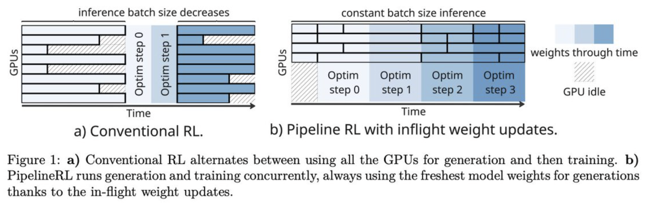Pipeline RL with in-flight weight updates Figure 10: Comparison of conventional RL and in-flight updating. From Pipeline RL paper.

In the context of Intellect-3, which uses a CPU orchestrator between two clusters (one for training and one for inference), the orchestrator continuously polls the trainer to update the inference pool once a new policy is available, and the inference pool temporarily halts generation to update the weights, then continues with rollouts. In this way, a long rollout could be generated by multiple policies, but they limit this by a max_off_policy_steps parameter to limit policy drift. Also, they implement IcePop to stabilize MoE training:

\[\mathcal{J}_{\text{IcePop}}(\theta)=\mathbb{E}_{x \sim \mathcal{D}, \{y_i\}_{i=1}^N \sim \pi_{\text{infer}}}\left[\frac1{\sum_{i=1}^N \lvert y_i \rvert} \sum_{i=1}^N \sum_{t=1}^{\lvert y_i \rvert}\left[\mathcal{M}\left(\frac{\pi_{\text{train}}(y_{i, t} \mid x, y_{i, <t>};\theta)}{\pi_{\text{infer}}(y_{i, t} \mid x, y_{i, <t>};\theta_{\text{old}})}; \alpha, \beta\right)\hat{A}_{i,t}\right] \right]\]

where $\mathcal{M}(k)=k$ if $k \in [\alpha, \beta]$ and $0$ otherwise. The purpose of $\mathcal{M}$ is to account for the off-policy nature between the training policy and the inference policy such that they don’t diverge significantly for each token. When the importance weight $k$ falls outside $[\alpha, \beta]$, $\mathcal{M}$ clips it to 0, effectively ignoring that token’s contribution to the gradient. This is the idea behind importance sampling, where rollouts come from the inference policy, but we are optimizing for the training policy. Prime uses the default $\alpha = 0.5, \beta = 5$. $\alpha$ and $\beta$ need not be symmetric in the multiplicative sense. One reason for this is under the rare instance when $\pi_\text{infer}$ is small (large $k$), a tighter $\beta$ would clip the high-entropy tokens, which would make learning dynamics worse.

Kimi K2 adapts a different policy optimization approach from their previous model K1.5:

\[L_\text{RL}(\theta) = \mathbb{E}_{x \sim \mathcal{D}}\left[\frac1{K} \sum_{i=1}^K\left[\left(r(x, y_i) - \overline{r}(x) - \tau \log\frac{\pi_\theta(y_i | x)}{\pi_\text{old}(y_i | x)}\right)^2\right]\right]\]

where $\overline{r}(x)= \frac1{K} \sum_{i=1}^K r(x,y_i)$ is the mean reward of sampled responses and $\tau > 0$ is a regularization parameter for stable learning, akin to KL divergence.

Another consideration is PTX loss: pre-training cross-entropy loss. During joint RL training, the model can catastrophically forget valuable, high-quality data. So, they curate a dataset using hand-selected, high-quality samples and integrate them into the RL objective via the PTX loss. The advantages are twofold: high-quality data can be leveraged, and the risk of overfitting to the tasks present during RL can be mitigated, which leads to better generalization.

To balance exploration and exploitation throughout training, they implement temperature decay. For tasks like creative writing and complex reasoning, high temperatures during the initial stages is important to generate diverse and innovative responses; this prevents premature convergence to local minima and facilitates the discovery of effective strategies. At later stages, the temperature is decayed (following a schedule) so that there is not excessive randomness, and that it doesn’t compromise the reliability/consistency of the model’s outputs.

DeepSeek-R1-Zero stands out as an exception compared to other models because it demonstrates that RL can be effective even without supervised fine-tuning. It cold-starts RL (specifically, GRPO to save training costs; they use 10.4k steps, batch size of 512, reference policy replacement every 400 steps along with lr as 3e-6, KL coefficient as 0.001) on reasoning tasks without any supervised data. The reward system uses two types of rewards: accuracy rewards based on correctness of the response and format rewards that enforce the model to put its thinking process between thinking tags. It obtains robust reasoning capabilities using pure RL, which validates the ability to learn reasoning and generalize effectively. Moreover, behaviors including reflection (re-evaluating previous steps) and exploring alternative approaches to problem-solving emerge, which further enhances reasoning. The count of reflective words such as “wait” or “mistake” rises 5-7-fold compared to the start of training. Moreover, this reflective behavior appeared relatively suddenly: between steps 4k-7k, there was only occasional usage, but after step 8k, it exhibited significant spikes.

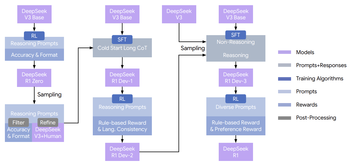
The multi-stage pipeline of DeepSeek-R1

Figure 11: The multi-stage pipeline of DeepSeek-R1 with intermediate checkpoints DeepSeek-R1 Dev1, Dev2, and Dev3. From DeepSeek.

For DeepSeek-R1, they collect thousands of long CoT data to finetune the DeepSeek-V3-Base as the starting point for RL. From DeepSeek-R1-Zero, they learned that readability was an issue: responses sometimes mixed multiple languages or lacked markdown formatting for highlighting answers. They remedy the former by introducing a language consistency reward (portion of target language words in the CoT), and the latter by designing a readable pattern that includes a summary at the end of each response. They also perform a second RL stage aimed at improving the model’s helpfulness and harmlessness while retaining reasoning capabilities.

For helpfulness, they focus on emphasizing the utility and relevance of the final summary. To generate preference pairs, they query DeepSeek-V3 four times and randomly assign responses as either Response A or Response B; they then average the independent judgments and retain pairs where the score difference is sufficiently large and use a pairwise loss to define the objective. For harmlessness, they evaluate the response to identify and mitigate any potential risk, biases, or harmful content. Using a dataset with model-generated responses annotated as “safe” or “unsafe” according to safety guidelines, the reward model is trained using a point-wise methodology to distinguish between safe/unsafe responses.

Impressively, they found that distilling DeepSeek-R1’s outputs into smaller models like Qwen-32B significantly improved reasoning capabilities, even compared to large-scale RL, which further requires significantly more compute. Moreover, it shows that even while distillation strategies are effective and economical, we will increasingly require more powerful base models and larger-scale RL.

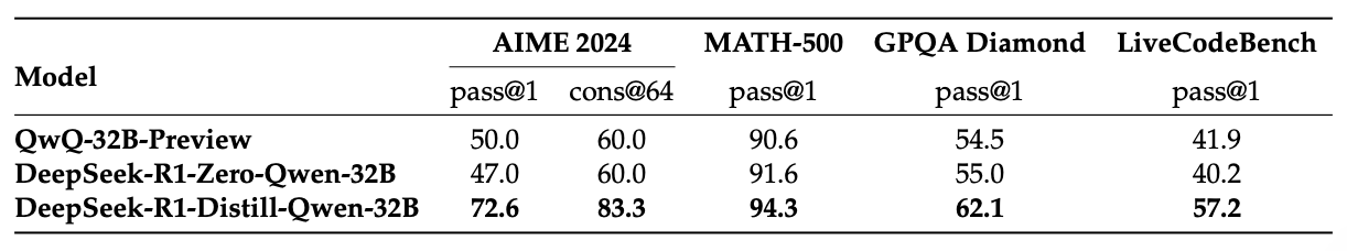
Comparison of DeepSeek-R1-distilled and RL Models on Reasoning-Related Benchmarks

Figure 12: Comparison of DeepSeek-R1-distilled and RL Models on Reasoning-Related Benchmarks. From DeepSeek.

Beyond the main training pipeline, DeepSeek’s appendix documents additional considerations that influenced their design choices:

GRPO over PPO: PPO has a per-token KL penalty (the KL between sequence distributions decomposes into a sum over time of KL between tokens, given the autoregressive nature). Because RL does enable longer reasoning over time and PPO implicitly penalizes the length of the response (and is less computationally expensive due to not needing an additional value model), GRPO is preferable; on MATH tasks, GRPO consistently performed better than PPO with $\lambda=1.0$, which further consistently performs better than PPO with $\lambda=0.95$.
product-driven DeepSeek-R1: users find responses more intuitive when the reasoning process aligns with first-person thought patterns. So, after finetuning on a small amount of long CoT data, DeepSeek-R1 uses “I” more whereas DeepSeek-R1-Zero uses “we” more. Other considerations were previously mentioned, like language consistency while ensuring CoT remains coherent and aligned. The raw CoT produced by DeepSeek-R1-Zero may have possessed potential beyond limitations of current human priors, so human annotators convert the reasoning trace into one that is more human-interpretable/conversational.
temperature for reasoning: they observed that greedy decoding to evaluate long-output reasoning models resulted in higher repetition rates and more variability. This coincides with recent research, and it can be explained by risk aversion due to hardness of learning and inductive bias for temporally correlated errors, which describes that at decision points, the model tends to reselect previously favored actions (resulting in looping).

RLVR and rubrics

The goal of RLVR on hybrid reasoning models is to improve reasoning capabilities without extending the token count too radically. For /no_think, naively applying GRPO can lead to reward hacking since the model begins to emit longer CoT (shifting towards /think); as such, both reward and token length increase. SmolLM3 observed this and found that RLVRed /no_think traces showed cognitive behaviors like “Wait, …” associated with reasoning models.

This can be mitigated via an overlong completion penalty which penalizes completions over a certain length, which is a function parametrized by a soft punishment threshold and a hard punishment threshold/max completion length. Penalty increases from the soft to the hard threshold, and past the latter, the punishment is -1 (effective reward = 0).

For /no_think, SmolLM3 decided on a length penalty in the range of 2.5k-3k that balanced improvement in performance and increase in response length. However, doing RL jointly on hybrid reasoning models is difficult since it requires separate length penalties, whose interplay can cause instability. This is also why labs release instruct and reasoning variants separately.

Kimi K2 uses a self-critique rubric reward mechanism, where the model evaluates its own outputs to generate preference signals. The K2 actor generates $k$ rollouts, and the K2 critic ranks all results by performing pairwise evaluations against a combination of rubrics; these combine core rubrics (fundamental values) and prescriptive rubrics (aimed to eliminate reward hacking), and human-annotated rubrics (for specific instructional contexts).

The critic model is refined using verifiable signals, and this process of transfer learning grounds its more subjective judgments in verifiable data. This should allow the critic to recalibrate its evaluation standard in lockstep with the policy’s evolution.

online data filtering

To RL effectively, curriculum learning is another effective way which gradually exposes the model to progressively difficult problems. First, problems are sorted into difficulty pools (such as easy, medium, and hard) based on the problem’s observed solve rate; In Intellect-3 for math and coding, this was done via querying Qwen/Qwen3-4B-Thinking-2507 over eight generations per problem while for science and logic, they queried the same model 16 times. Then, during each stage, they maintain a balanced curriculum that avoids training with trivially easy or overly difficult problems which don’t give meaningful learning signal (and also helps maintain gradients in GRPO). In Kimi K2, this was done by using the SFT model’s pass@k accuracy.

alternatives to RL

One alternative is online DPO (see “On policy with grading” in the preference optimization section). Another is on-policy distillation. Instead of preferences, the signal comes from a stronger teacher model, where the student samples responses at every training step and the KL divergence between the student/teacher logits provides the learning signal. That way, the student can continuously learn from the teacher. Also, on-policy distillation is much cheaper than GRPO since instead of sampling multiple rollouts per prompt, we only sample one, which is graded by the teacher in a single forward-backward pass; its performance boost, as the Qwen3 tech report notes, can be larger across the board as well. One limiting factor is that the student and the teacher must share the same tokenizer, and Hugging Face’s General On-Policy Logit Distillation (GOLD) allows any teacher to be distilled into any student.

Thinking Machine’s blog further showed that on-policy distillation mitigates catastrophic forgetting, where a model post-trained on a new model regresses on other, previous domains. Specifically, they found that mid-training 70% and with on-policy distillation can achieve close to the best performance of a model and its mid-trained version, effectively restoring behavior with cheap distillation.

Given these aforementioned algorithms, choosing between them can be hard; Hugging Face aptly describes it:

Algorithm	When to Use	Tradeoffs	Best for Model Size
Online DPO	You can get preference labels cheaply. Best for aligning behaviour with evolving distributions.	Easy to scale iteratively, more stable than RL, but depends on label quality and coverage. Supported in few training frameworks.	Any size, where preferences capture improvements beyond imitation.
On-policy distillation	You have access to a stronger teacher model and want to transfer capabilities efficiently.	Simple to implement, cheap to run, inherits teacher biases, ceiling limited by teacher. Supported only in TRL and NemoRL	Most effective for small to mid-sized models (<30B).
Reinforcement learning	Best when you have verifiable rewards or tasks requiring multi-step reasoning/planning. Can be used with reward models, but there are challenges like reward-hacking, where the model takes advantage in weaknesses in the reward model.	Flexible and powerful, but costly and harder to stabilise; requires careful reward shaping. Supported in most post-training frameworks.	Mid to large models (20B+), where extra capacity lets them exploit structured reward signals.

And for DPO (semi-online and online), it is also possible to match GRPO using far less compute. Specifically, they found that semi-online DPO (with syncing between the trainer and the generator every 100 steps) was generally the best compared to semi-online DPO with sync every 10 steps, online DPO, and GRPO.

limitations

DeepSeek shares other experimental methods when developing DeepSeek-R1 that ultimately failed. Monte Carlo Tree Search (MCTS), inspired by AlphaGo and AlphaZero, was implemented to test enhancing test-time compute scalability. This breaks answers into smaller parts to allow the model to explore the solution space systematically. To do this, they prompted the model to generate tags corresponding to reasoning steps necessary. The problem is that token generation exists in an exponentially larger search space compared to chess. So, they set a max extension limit for each node, but this leads to the model getting stuck in local optima. Moreover, training a fine-grained value model is difficult, also due to complexities of token generation.

They also explored process reward models, which rewards intermediate thoughts in multi-step tasks. DeepSeek acknowledges three limitations: defining a fine-grained step in general reasoning is difficult, determining whether the current intermediate step is difficult (LLM-as-judge might not yield satisfactory results), and it leads to reward hacking because the model would optimize for the appearance of good reasoning without doing the underlying work.

behaviors and safety

safety testing and mitigation

During post-training, they perform an additional stage of RL to reward answers that comply with OpenAI’s policy against unsafe prompts. Because all of these models have open model weights, then one worry is that malicious parties can enhance the model’s harmful capabilities. By running Preparedness evaluations on gpt-oss-120b, OpenAI confirmed that the model doesn’t achieve threshold for high capability in biological/chemical capability, cyber capability, and AI self-improvement.

They also tested whether adversarial actors could fine-tune gpt-oss-120b to reach high capability in the aforementioned domains. They simulated the attack by either:

evaluating the model in collegiate Capture the Flag challenges or cyber operations in a realistic, emulated network
creating adversarially fine-tuned versions via incrementally training it on in-domain human expert data related to biorisk
benchmarking on SWE-bench verified, OpenAI PRs, and PaperBench (ability to recreate AI research)

Upon review, their safety advisory group concluded that even with robust fine-tuning, gpt-oss-120b still couldn’t reach high capability in the aforementioned domains. Also, they determined whether releasing the model could advance the frontier of biological capabilities, including evaluations like virology and tacit knowledge, in open foundation models (which also increases risk) and found that there were other open weight models at or near gpt-oss-120b, so they decided that releasing has low impact on the frontier.

OpenAI also evaluated safety performance using other indicators:

Disallowed content: benchmarked on ProductionBenchmarks, they consider different categories such as PII, sexual, harassment, hate, self-harm using conversations more representative of production data. They evaluate completions using LLM-as-judge and determine not_unsafe according to the relevant OpenAI policy. Performance is on par with o4-mini.
Jailbreaks: they test with adversarial prompts that try to circumvent model refusals, specifically StrongReject which inserts jailbreak examples into the safety refusal eval and also uses the same policy grader. Performance is on par with o4-mini.
Instruction Hierarchy: it follows system > developer > user > assistant > tool. They post-trained the model using system, developer, and user messages, sometimes conflicting, and the model must learn to choose the instruction higher in the hierarchy. This includes testing system prompt extraction via a user message and prompt injection hijacking. For PII protection, performance is on par with o4-mini, but for message conflict, gpt-oss-120b underperforms o4-mini by ~15%.
Hallucinations and CoT: reasoning model’s CoT can be very helpful for detecting misbehavior, and that models could learn to hide their thinking while misbehaving when pressured against having “bad thoughts.” To measure hallucinations, they use two datasets of either fact-seeking questions or publicly available facts about people and consider accuracy and hallucination rate. Here, hallucination rate is not just defined as 1 - accuracy, since the model can also output answers like “I don’t know.” Performance is a bit worse than o4-mini, which is expected given model size.
Fairness and Bias: they also evaluate gpt-oss-120b on the BBQ evaluation which tests social bias against people belonging to protected classes along nine social dimensions. Performance is on par with o4-mini.

behaviors and latent capabilities

Continuing from the chat template section, Nous’ decision to change the token used from the assistant’s turn from $\mathtt{assistant}$ to $\mathtt{me}$ enabled Hermes 4 to adopt a first-person, peer-like persona. Hermes 4 generates responses with fewer meta-disclaimers and more consistent voice embodiment, resulting in higher behavioral plasticity that is not as common in large models.

Similarly, Hermes 4 demonstrates comparatively greater contextual fidelity over policy rigidity. Most other large models will follow policy compliance even when faced with fictional or controlled prompts (such as issuing disclaimers or reformulated responses to align with safety constraints), but Hermes 4 interprets fictional prompts more as role-play and generates in-character responses. This also means that Hermes 4 has a lower refusal rate; on their internal RefusalBench, they found that Hermes 4 (reasoning) ranked highest (lowest refusal rate) among all tested models, whereas gpt-oss-120b and gpt-oss-20b, perhaps unsurprisingly, had the lowest scores (highest refusal rate). Also, this level of embodied personas extends even to political analysis, where the model produces reasoning balancing factual recall with nuanced framing, and less of policy-driven hedging common to other large models.

Excessive sycophancy is an undesired behavioral trait, so most models apply an anti-sycophancy system prompt to adjust surface-level politeness while leaving underlying reasoning unchanged. When implemented in Hermes 4, Nous observed a deeper shift: CoT traces reflect the aim to steer user interaction away from inference. This sometimes introduces embodied or emphatic language.

the training marathon

Before the main training run starts, ensure the infrastructure is ready. This includes Slurm reservations on clusters, stress-testing GPUs (GPU Fryer or DCGM), and avoid storage bloat by uploading checkpoints to third parties and deleting local copies after saving the next. To this end, checkpoint and auto-resume systems are important.

Evals are also deceptively time-consuming (Allen Institute spent roughly 20% on compute on evals), so ensuring automation and logging (not just evaluation scores, but also throughput, loss, gradient norm, and node health) is crucial.

vanishing throughput

Hugging Face observed a ~40% drop in throughput (14k to 8k tokens/sec/GPU) after a few hours of starting the main run. The issue came from data storage; their cluster uses a network-attached storage with a “keep-hot” caching model that stores frequently accessed files and evicts “cold” files to third-party S3. With 24TB of training data, the storage was pushed to its limit, so it evicted dataset shards mid-training. This meant fetching them back and creating stalls that slowed throughput.

The first fix came in the form of swapping the storage method by reserving a spare node with the dataset preloaded and copying using fpsync (s5cmd took double the time). This fixed the issue of a node dying and the replacement GPU having no data since by swapping it with the spare node, training could continue. So, the new spare, not to be wasted, could run evals or dev jobs.

Testing again, they found smaller but still prominent drops in throughput. After experimenting with individual nodes that yielded the same result, they focused on the change in training steps and found that smaller step counts resulted in smaller throughput drops. The nanotron dataloader they were using was growing the lookup table making the training step to the next chunk of tokens to read instead of keeping it bounded or precomputed. Stored in global memory, the growing table causes allocation failures and page faults/worse cache locality. So, they switched to Tokenizedbytes dataloader, solving the throughput issue.

noisy loss

However, the loss curve for SmolLM3 looked more noisy. They found the issue with the dataloader because it reads sequences sequentially for each document. Without shuffling of sequences, batches are no longer representative of the overall data distribution, increasing gradient variance. Also, a long file (e.g. code) would supply many consecutive sequences that would also spike loss. To fix, they reshuffled the tokenized sequences offline; an alternative was changing the dataloader to do random access, which has both higher memory usage and slower runtime.

tensor parallelism

After two days and 1T tokens, evals showed that with a similar recipe, SmolLM2 (1.7B) was more performant at the same stage in training as SmolLM3 was. The team found the issue with tensor parallelism: the weights of SmolLM2 fit on a single GPU, whereas for SmolLM3, they had to be shared across 2 GPUs.

Further, the two TP ranks were initialised with the same random seed instead of different seeds, which causes similar activations/gradients, a loss of diversity of features, and lower convergence.

multi-client orchestrator

Inference throughput should scale linearly with the number of nodes used. However, Prime found that the standard multi-node data-parallel strategy provided by vLLM didn’t deliver this because as nodes increased, throughput plateaued. They abstracted the multi-client orchestrator so that each inference node is deployed on an independent server (runs its own vLLM engine and scheduler, manages its own KV cache and batches its own requests), and the orchestrator maintains one client per node (avoids single-shared queue bottleneck). Groups rollout requests are distributed across clients according to round-robin scheduling, which keeps utilization balanced.

the usual suspects

There are a few common culprits for training instabilities: high learning rate, bad data, data-parameter state interactions (spikes can come from specific combinations of data batches and model parameter states), poor initialisation (OLMo2 revealed that $\mathcal{N}(0, 0.02)$ can improve stability upon scaled initialisation), and precision (eww, not fp16).

Besides aforementioned ideas like z-loss or QKNorm, data filtering (OLMo2 removed documents with repeated n-grams, specifically those with 32+ repetitions of 1-13 token spans) significantly reduces spike frequency. If spikes still occur, common methods include retraining around the spike by skipping problematic batches or tightening gradient clipping.

activation engineering for privacy protection in LLMs

paper reading catalog

general practices

architecture and set-up

attention

document masking

embedding sharing

positional encodings

attention for long contexts

MoE

hybrid models

stability

$z$-loss

removing weight decay from embeddings

qk norm

other design considerations

tokenizer

optimizers and training hyperparameters

adamW

muon

learning rates

batch size

scaling laws

data curation and pre-training

multi-stage training

ablation

token utility

pre-training data

SmolLM3

hermes 4

mid-training

post-training

evals

post-training data

intellect 3

hermes 4

kimi k2

chat template

sft

capabilities

sequence packing

learning rate and epochs

preference optimization (PO)

algorithms

RL

RLVR and rubrics

online data filtering

alternatives to RL

limitations

behaviors and safety

safety testing and mitigation

behaviors and latent capabilities

the training marathon

vanishing throughput

noisy loss

tensor parallelism

multi-client orchestrator

the usual suspects