combinatorial reasoning environments for LLMs and RL
Can RL agents learn to play spatial reasoning puzzle games as well as, or better than, LLMs? We develop a complete RL pipeline by developing an environment for fruit box (a grid-based reasoning game) using Prime Intellect’s verifiers library, benchmarking LLMs like gpt-5.1 and gemini-3-pro, and training RL agents with SFT and GRPO to play. Repo here.
This blog is structured chronologically. First, writing scripted policies that reveal strategy and help validate the core environment mechanics. Second, developing the environment and integrating it with Prime Intellect’s verifiers library to create an LLM-facing eval framework. Third, evaluating reasoning models against expert-level performance. Finally, post-training RL agents using both pure modified GRPO and SFT while exploring two training paradigms related to masking and the learning problem. This blog also represents a valuable lesson in engineering pragmatism.
Update (Nov 12th): The environment was merged into the prime-environments repo, thanks Christian and Sinatras!
tl;dr
- counterintuitive strategy: Minimizing cleared cells (mean 113.72, 81.7% win rate) significantly outperforms maximizing them (mean 97.61, 3.2% win rate) in Fruit Box, a grid-based spatial reasoning puzzle
- RL beats LLMs: Specialized RL agent achieves 94.4% performance (relative to expert), outperforming the best reasoning LLMs (
Qwen3-235b-thinkingat 84.6%,gpt-5at 83.5%) by ~10 percentage points - pragmatism wins: The purist approach (learning legality constraints from scratch) struggled to achieve consistent legality, while the pragmatic approach (legal masking) achieved 107.3 average score, just 6 points below the expert policy (113.72)
- LLMs can reason spatially: Despite the gap, reasoning LLMs achieve 80%+ performance, suggesting they can handle spatial reasoning tasks, just not as precisely as specialized architectures
fruit box and intuition
Fruit Box is played on a 10×17 board where each cell contains a digit 1-9. The objective is to clear as many cells as possible by selecting rectangular regions that sum to exactly 10. If valid, those cells are cleared and the player earns points equal to the number of non-zero cells cleared in that move. Here’s an insanely good person playing the game:
Why? The game requires spatial reasoning, combinatorial search, and strategic planning—capabilities where LLMs and RL agents often struggle. Unlike many benchmark environments, Fruit Box has a large, $\binom{10+1}{2}\cdot\binom{17+1}{2}=8415$, discrete action space, making it a good testbed for evaluating different learning paradigms. The game also has clear optimal strategies (as we’ll see), allowing me to compare learned policies against known baselines. Additionally, the multi-turn nature and the need to reason about future moves make it particularly well-suited for studying how LLMs and RL agents handle constrained sequential decision-making.
The game is quite fun, admittedly addictive, for its simplicity. Initially, I assumed higher scores required faster scanning, but simple games often have ‘cool tech’. One example that comes to mind is the 2048 game, where speedrun strategies always put the biggest tile in a corner (e.g. bottom-right) then button-mash arrows (e.g. down and right) to quickly accumulate large tiles. After playing several rounds, I developed key intuitions that motivate the scripted policies:
- pairings: 1’s must go with 9’s, so 1’s should be used sparingly. Similarly, 2’s usually go with 8’s; occasionally, it makes sense to select 1—1—8 over 2—8.
- greediness: A corollary is that the greedy algorithm is bad because it will try to find a rectangle using as many digits, increasing the likelihood of using 1’s or 2’s without pairing it with 9’s and 8’s. In fact, I found that the opposite of greedy (a minimal approach) is very effective.
- low-level tech: patterns that are clearable only a certain way. For example, clearing the middle 9—1 instead of the first-column 1—9 because in the later case, the leftover 1 and 9 can’t be cleared.

- time-saving: I find it helpful to search for the next rectangle while clearing the current one. This probably saves ~0.2 seconds per rectangle, but across the ~50 rectangles cleared, this saves ~10 seconds.
- non-systemic: this is person-specific, but systematic search (like starting in the top-left and working row-by-row while checking columns) is algorithmically faster due to less redundancy with overlapping cells, but it helped just to let my eyes naturally wander, clearing nearby rectangles.
scripted policies
With this in mind, there are 4 policies that are of interest:
- random: choose a legal rectangle randomly. This serves as a sort of “baseline.”
- greedy: choose the legal rectangle that maximizes cells cleared.
- 2-step lookahead: choose the legal rectangle that maximizes a discounted $Q$-value.
- minimal: choose the legal rectangle that minimizes cells cleared.
There’s a nuance to grid generation: each cell is distributed multinomially across the 9 digits, but the total sum across all 170 cells must be a multiple of 10. This is to allow a perfect clearing, though many grid configurations may be impossible to perfect, e.g. if the number of 9’s is greater than the number of 1’s. To generate valid grids, I continuously sample sequences (10 expected) until the sum is a multiple of 10.
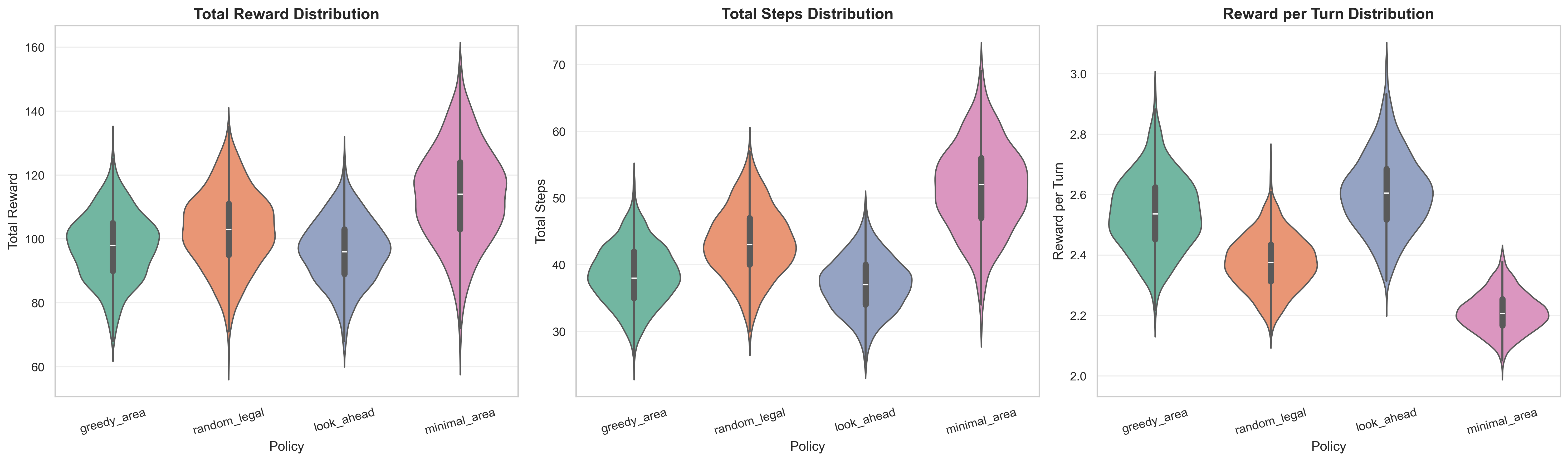
I generated 1000 seeds and benched the four policies:
| Policy | Mean | Std |
|---|---|---|
| greedy | 97.61 | 10.53 |
| random | 102.89 | 12.04 |
| 2-step lookahead | 96.22 | 10.05 |
| minimal | 113.72 | 14.89 |
All four policies had roughly the same minimum score, but the minimal area policy had 5 runs that scored over 150, achieving a maximum of 157. We note a few insights:
-
minimal beats greedy: the minimal policy (mean 113.72) significantly outperforms greedy (mean 97.61), confirming my intuition that preserving 1’s and 2’s for later use is crucial. But can an RL agent learn this delayed gratification strategy?
-
lookahead provides minimal benefit: the 2-step lookahead policy (mean 96.22) performs slightly worse than greedy. This is probably because short-term lookahead isn’t sufficient to capture the strategic value of preserving small numbers. This is somewhat surprising but makes sense given the context of the minimal strategy.
-
random is competitive: random (mean 102.89) as a baseline outperforms both greedy and lookahead, which seemed initially counterintuitive but shows how greedy strategies can be locally optimal but globally suboptimal.
-
minimal clears (figuratively and literally): to hit the nail on the head, I tested win-rate of the 4 policies across the 1k seeds. Minimal had a stellar win-rate of 81.7%, followed by random at 13.7%, greedy at 3.2%, and 2-step lookahead at 1.4%.
The trajectory data logged while benching the four policies is (roughly) summarized below:
{
  episode_id: string,
  step: int,
  grid: List[List[int]],  # 10x17 grid state
  action: {"c1": int, "c2": int, "r1": int, "r2": int},
  num_legal_actions: int,
  reward: int,
  done: bool,
  agent_tag: string,
}
The data was uploaded here in full and here just for minimal.
creating the environment
With validated policies and trajectory data in hand, we’re now ready to build the environment using Prime Intellect’s verifiers library. The verifiers framework structures environment creation into six key components: data, interaction style, environment logic, rewards function, parser, and packaging. The actual implementation is 550 lines long, so we provide an abbreviated version, keeping the core functionality of each component. This section’s organization is inspired by Yacine’s video.
1. data
We load episodes from HuggingFace datasets and format them into the verifiers’ expected structure such that each example contains an initial prompt with the game rules and grid state, along with ground truth trajectory information. We group rows by episode_id and agent_tag to reconstruct complete trajectories, then constructs prompts by combining game rules with the starting grid state encoded as JSON. The "info" field preserves the expert’s total reward for later score normalization.
Show code
GAME_RULES = textwrap.dedent("""...""")

def build_dataset() -> Dataset:
    hf_dataset = load_dataset(dataset_name, split=dataset_split)

    # group trajectories by episode_id and agent_tag
    episodes = {}
    for row in hf_dataset:
        ep_id = row["episode_id"]
        agent_tag = row.get("agent_tag", "unknown")
        key = f"{ep_id}_{agent_tag}"
        if key not in episodes:
            episodes[key] = []
        episodes[key].append(row)

    # build examples with initial prompt and ground truth
    data = []
    for key, trajectory in episodes.items():
        initial_state = trajectory[0]
        initial_grid = initial_state["grid"]
        total_reward = sum(step.get("reward", 0) for step in trajectory)

        grid_json = json.dumps({"grid": initial_grid})
        initial_prompt = f"{GAME_RULES}\n## Initial Grid State\n{grid_json}\n What move do you make?"

        data.append({
            "prompt": [{"role": "user", "content": initial_prompt}],
            "answer": json.dumps({"trajectory": ground_truth_actions, ...}),
            "info": {"initial_grid": initial_grid, "total_reward": total_reward, ...}
        })

    return Dataset.from_list(data)
The dataset serves two key purposes during evaluation. First, it provides test cases across different initial grid states. Second, it supplies ground truth for normalization: the "info" field stores the expert’s total_reward on that initial grid, which the rubric (covered later) uses to normalize LLM performance scores. This normalization is crucial because different initial grids have different maximum achievable scores—some grids are inherently easier or harder to clear completely.
2. interaction
The verifiers library provides a lovely multi-turn interaction between the environment and the LLM to exchange messages. We inherit from MultiTurnEnv and implement the env_response method, which processes the LLM’s JSON-formatted move and returns the updated game state. The async method extracts the last assistant message to get the current move, executes it on a fresh Sum10Env instance, then returns a JSON response with validity, reward, and the updated grid state.
Show code
class FruitBoxEnv(MultiTurnEnv):
    async def env_response(self, messages: Messages, state: State, **kwargs) -> Tuple[Messages, State]:
        assistant_messages = [m for m in messages if m["role"] == "assistant"]
        turn_num = len(assistant_messages)

        # parse last assistant message to extract action
        last_content = assistant_messages[-1]["content"]
        parsed = json.loads(last_content)
        action = parsed.get("action", {})
        r1, c1, r2, c2 = action.get("r1"), action.get("c1"), action.get("r2"), action.get("c2")

        # execute move
        current_grid = state.get("current_grid", state["info"]["initial_grid"])
        env = Sum10Env()
        env.reset(grid=np.array(current_grid))
        step_info = env.step(r1, c1, r2, c2)

        # update state and return
        state["current_grid"] = env.grid.tolist()
        response = {
            "valid": step_info.valid,
            "reward": step_info.reward,
            "done": step_info.done,
            "grid": env.grid.tolist()
        }
        return [{"role": "user", "content": json.dumps(response)}], state
3. logic
The core game logic lives in Sum10Env, which manages grid state, validates moves, and computes rewards. It uses prefix sums for efficient rectangle sum queries, allowing O(1) rectangle queries across all $8415$ combinations. The step function validates coordinates, checks that the sum equals 10, clears cells, and determines game termination.
Show code
class Sum10Env:
    def __init__(self):
        self.grid = np.zeros((10, 17), dtype=np.uint8)
        self.turn = 0
        self.sum = None  # prefix sum
        self.count = None

    def rebuild_prefix_sums(self):
        self.sum = self.grid.astype(np.int32).cumsum(axis=0).cumsum(axis=1)
        non_zero = (self.grid > 0).astype(np.int32)
        self.count = non_zero.cumsum(axis=0).cumsum(axis=1)

    def step(self, r1, c1, r2, c2) -> StepInfo:
        # normalize
        if r1 > r2: r1, r2 = r2, r1
        if c1 > c2: c1, c2 = c2, c1

        # validate bounds and sum
        if not (0 <= r1 <= r2 < 10 and 0 <= c1 <= c2 < 17):
            return StepInfo(valid=False, sum=0, reward=0, done=True)

        s = self.box_sum(r1, c1, r2, c2)  # rectangle sum via prefix sums
        reward = self.box_nonzero_count(r1, c1, r2, c2)

        if s != 10 or reward == 0:
            return StepInfo(valid=False, sum=s, reward=0, done=False)

        # clear cells and update
        self.grid[r1:r2+1, c1:c2+1] = 0
        self.rebuild_prefix_sums()
        self.turn += 1
        done = not self.has_any_legal()  # check if any valid moves remain

        return StepInfo(valid=True, sum=10, reward=reward, done=done)
4. rewards
The rubric defines how we evaluate LLM performance. Our reward_total_score function replays the LLM’s trajectory and computes the total score, normalized by expert (minimal-area policy) performance. This provides a score between 0.0 and 1.0, where 1.0 indicates matching or exceeding the expert’s performance. The function deterministically replays each move from the initial grid state, accumulating rewards for valid moves and stopping on the first invalid move. Normalization by expert performance accounts for grid difficulty, making scores comparable across different initial configurations.
Show code
def reward_total_score(completion: List[dict], state: dict, **kwargs) -> float:
    initial_grid = state["info"]["initial_grid"]
    env = Sum10Env()
    env.reset(grid=np.array(initial_grid))

    total_reward = 0
    assistant_messages = [m for m in completion if m["role"] == "assistant"]

    for msg in assistant_messages:
        action = parse_action(msg["content"])
        if action is None:
            continue

        step_info = env.step(action.get("r1"), action.get("c1"),
                            action.get("r2"), action.get("c2"))

        if step_info.valid:
            total_reward += step_info.reward
        else:
            break  # invalid move ends trajectory

        if step_info.done:
            break

    # normalize by expert performance
    expert_reward = state["info"]["total_reward"]
    return min(1.0, total_reward / expert_reward) if expert_reward > 0 else 0.0
The rubric is solely dependent on the normalized trajectory, but it could be expanded by adding other factors like penalizing excessive turns, invalid moves, etc.
5. parser
The parser extracts structured actions from LLM responses. A lightweight regex to find JSON objects within the response suffices. It first attempts a direct JSON parse, then falls back to regex extraction if the response contains explanatory text or markdown. The parser validates that all required coordinate fields are present and handles a special “no valid moves” signal with coordinates (-1, -1).
Show code
def parse_action(content: str) -> Optional[Dict]:
    try:
        # Try direct JSON parse first
        parsed = json.loads(content)
    except json.JSONDecodeError:
        # o.w, use regex
        import re
        json_match = re.search(r"\{.*\}", content, re.DOTALL)
        if json_match:
            parsed = json.loads(json_match.group())
        else:
            return None

    action = parsed.get("action", {})
    if all(k in action for k in ["r1", "c1", "r2", "c2"]):
        # Check for "no valid moves" signal
        if action.get("r1") == -1 and action.get("c1") == -1:
            return None
        return action
    return None
6. packaging
The load_environment function ties all components together, creating a complete verifiers environment ready for evaluation or training. It combines the dataset, environment class, and rubric into a single vf.Environment object. The max_turns ($\frac{170}{2}=85$) parameter prevents infinite loops by capping the maximum number of moves per game, which is especially important to prevent reasoning loops. Not having this initially will come to bite me later, though.
Show code
def load_environment(
    dataset_name: str = "djdumpling/fruit-box-minimal-area",
    dataset_split: str = "train",
    max_turns: int = 85,
    seed: Optional[int] = None,
) -> vf.Environment:
    # Build dataset from HuggingFace
    dataset = build_dataset()

    # Create rubric with reward function
    rubric = vf.Rubric(funcs=[reward_total_score], weights=[1.0])

    # Instantiate environment
    env_instance = FruitBoxEnv(
        max_turns=max_turns,
        dataset=dataset,
        rubric=rubric,
    )

    return env_instance
benchmarking
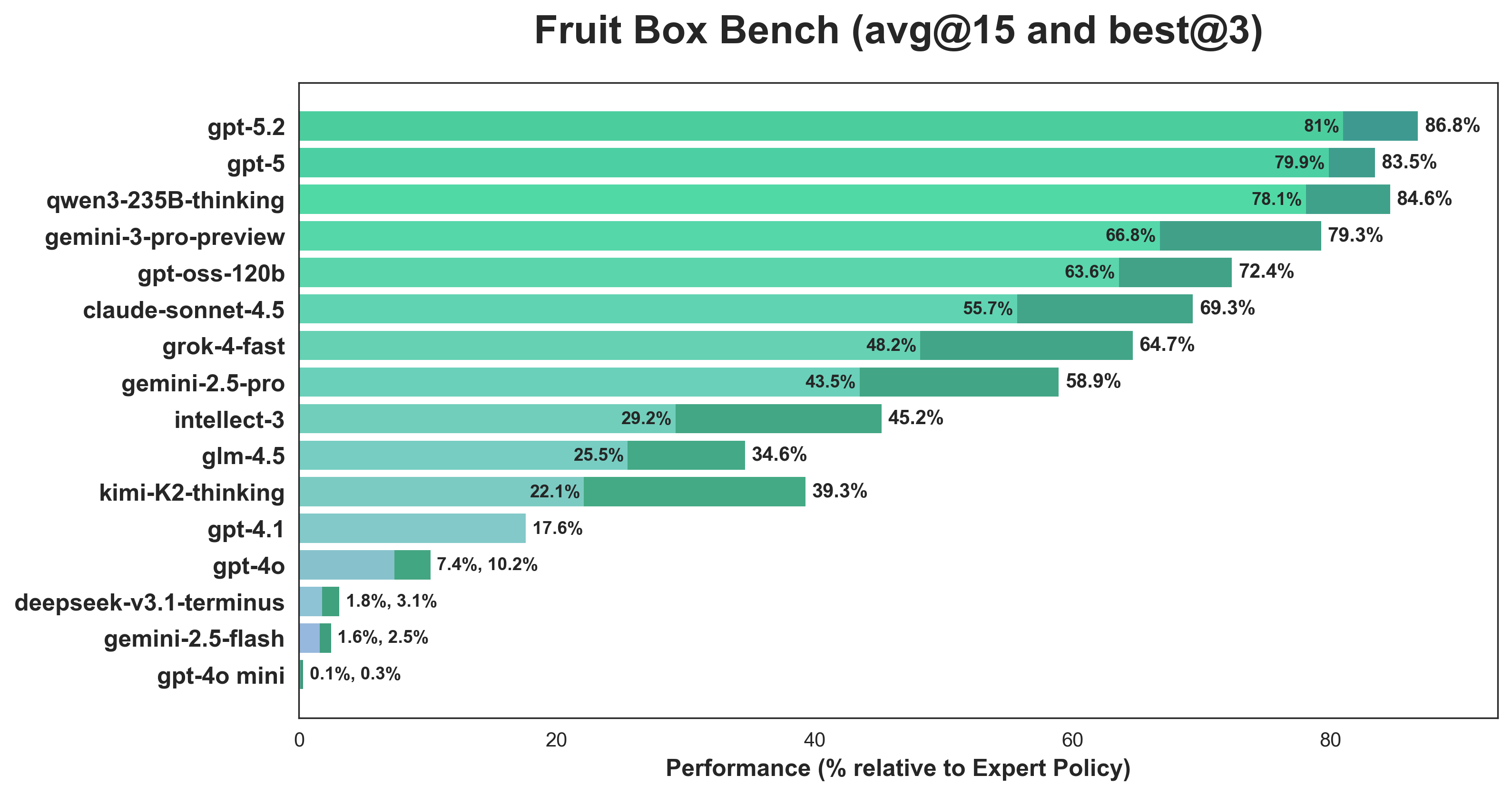
We’re now ready to benchmark different LLMs on Fruit Box. We benchmark using avg@15 and best@3: using the first 5 seeds (from the huggingface dataset), we evaluate each 3 times and either average all 15 or average the best from each of the 3 rollouts. All models perform text-based reasoning only: they receive the board state as text and must reason through moves without tools, code, or external computation. All LLM inference was conducted via Prime Intellect’s hosted inference.
non-reasoning LLMs
We first tested on a suite of non-reasoning models including gpt-4o, gpt-4o-mini, and gpt-4.1. The first two never progressed beyond the second move, often failing to make an initial valid move. gpt-4.1 performed the best, with a mean of ~20 and a maximum of 44. This is substantially below even the random policy baseline, which can roughly be explained by
-
formatting: The non-reasoning models sometimes fail to output the required JSON format, leading to parsing issues that ended runs early. This is either a symptom of a non-rigorous prompt or a lack of general instruction-following.
-
planning: They roughly follow a systematic search, sweeping top-left to bottom-right and always choosing the first legal rectangle they see. Many moves are only possible after clearing neighboring cells, and non-reasoning models neglect this.
Initially, we simply paste the board state and ask the LLM to pick a move. To remedy the planning problem, we modified the prompt to explicitly list all possible legal rectangles and ask the LLM to choose from that list, which improved the mean up to 70. This shows that providing explicit candidate moves helps non-reasoning models perform much better, though they still lack the ability to reason about which moves to prioritize strategically.
reasoning LLMs
Benched on a variety of models like gpt-5, qwen3-235b-thinking, gemini-3-pro, claude-sonnet-4.5, grok-4-fast, and variants, reasoning models (including hybrid reasoning models) are much more performant. The best reasoning models,gpt-5 and qwen3-235b-thinking, consistently achieved over 90, reaching a peak of 121 and 123, respectively. This is a bit misleading, because the bench uses the first 5 seeds, all of which the minimal-area policy achieved over 120 on. However, they are consistent as well: gpt-5 had an average standard deviation of 2.61, whereas qwen-3-235b-thinking’s average standard deviation was 6.52.
Mid-runners had more spotty performance: worse averages even without considering the high variance that ended some runs early. For example, on seed 2, gemini-3-pro scored $[38, 107, 118]$ and claude-sonnet-4.5 scored $[16, 74, 88]$.
CoT was hidden, but through the logs, we can get a small glimpse into their decision-making. The example from gpt-5 below shows two late-stage turns that illustrate how the LLM carefully verifies its moves:
=== Grid Visualization ===
 1  7  4  9  7  2  2  4  7  7  7  0  0  0  0  8  8
 0  0  9  7  8  0  0  0  0  6  0  0  0  9  7  7  1
 2  5  6  8  8  9  0  0  7  6  1  0  0  7  1  0  3
 9  3  0  6  6  9  0  0  2  9  0  0  0  0  0  0  4
 7  5  0  0  0  4  2  9  2  0  0  0  0  0  0  0  4
 0  0  0  0  0  8  0  0  0  0  0  0  0  0  0  0  1
 0  0  1  0  0  0  0  0  3  0  0  0  0  6  7  0  8
 0  0  0  0  0  0  0  8  0  0  0  0  0  0  0  0  5
 0  0  8  0  0  5  0  3  3  0  0  0  0  2  5  7  0
 0  0  3  5  0  0  0  0  0  6  0  9  0  6  0  0  0


=== Turn 43 ===
Action: (2,10) -> (9,11)
Reasoning: Identified a vertical rectangle from rows 2 to 9 and columns 10 to 11. Values: [(2,10)=1, (2,11)=0, (3,10)=0, (3,11)=0, (4,10)=0, (4,11)=0, (5,10)=0, (5,11)=0, (6,10)=0, (6,11)=0, (7,10)=0, (7,11)=0, (8,10)=0, (8,11)=0, (9,10)=0, (9,11)=9]. Sum = 1 + 9 = 10.
Candidate moves found: 1
  1. (2,10) -> (9,11)
Actual sum: 10
✓ Valid! Cleared 2 cells. Total: 103

=== Turn 44 ===
Action: (3,8) -> (8,8)
Reasoning: Examined column 8 for a zero-assisted vertical rectangle. From rows 3 to 8, the values are [2,2,0,3,0,3], which sum to exactly 10.
Candidate moves found: 2
  1. (3,8) -> (8,8)
  2. (6,2) -> (6,13)
Actual sum: 10
✓ Valid! Cleared 4 cells. Total: 107

=== Grid Visualization ===
 1  7  4  9  7  2  2  4  7  7  7  0  0  0  0  8  8
 0  0  9  7  8  0  0  0  0  6  0  0  0  9  7  7  1
 2  5  6  8  8  9  0  0  7  6  0  0  0  7  1  0  3
 9  3  0  6  6  9  0  0  0  9  0  0  0  0  0  0  4
 7  5  0  0  0  4  2  9  0  0  0  0  0  0  0  0  4
 0  0  0  0  0  8  0  0  0  0  0  0  0  0  0  0  1
 0  0  1  0  0  0  0  0  0  0  0  0  0  6  7  0  8
 0  0  0  0  0  0  0  8  0  0  0  0  0  0  0  0  5
 0  0  8  0  0  5  0  3  0  0  0  0  0  2  5  7  0
 0  0  3  5  0  0  0  0  0  6  0  0  0  6  0  0  0
legal action masks for LLMs
In a small follow-up experiment, we test providing reasoning LLMs with the complete set of all possible legal moves at each turn. This modification seems to have neutralized performance differences across models: grok-4-fast achieved 0.770, gpt-5.2 achieved 0.763, and grok-4 achieved 0.770. While these scores are close to top performance (~0.82), the convergence suggests that providing explicit move lists leads to strategy convergence: they default to selecting from the first moves in the list, which biases toward similar strategies regardless of model capabilities; another related reason is that they over-index on the provided list and rely less on strategic reasoning.
limitations and token efficiency
One notable limitation is computation time: just one run took ~1.2 hours, far beyond the 2-minute time limit, but it’s unfair to impose time constraints on LLMs since the objective is purely to benchmark LLM reasoning on games. Perhaps as inference time accelerates, it makes more sense to begin considering time constraints, or adding a criteria to the rubric that penalizes long thinking times.
To address the aforementioned standard deviation, we consider best@3 (across 3 rollouts, best score) and find that all models that are at least semi-performant improve significantly. Without the higher-variance runs weighing it down, qwen3-235b-thinking beats gpt-5 84.6% to 83.5% while being over 3 times cheaper for inference.
On that note, understanding token efficiency of LLMs is interesting; Nous Research has this nice blog on this. This probably isn’t great metric because it confounds with reasoning depth (like when the model systematically checks its work). We also consider time efficiency but ignore the least-3 performant models (deepseek-v3.1-terminus, gemini-2.5-flash, and gpt-4o-mini) as well as other models of the same class and provider (e.g. gpt-5 reasonably covers gpt-5.1 and gpt-5.2). All inference costs and timing data below are from Prime Intellect’s hosted inference (multi-turn with reasoning is very expensive 😞):
| Model | Avg Reward | Time (min) | Time Efficiency | Cost ($) | Tokens (M) | Token Efficiency |
|---|---|---|---|---|---|---|
| gpt-5 | 0.798 | 66.33 | 1.55 | $79.21 | 7.92 | 12.98 |
| qwen3-235b-thinking | 0.781 | 244.05 | 0.412 | $20.31 | 6.77 | 14.86 |
| gemini-3-pro | 0.668 | 61.70 | 1.39 | $77.96 | 6.50 | 13.23 |
| gpt-oss-120b | 0.636 | 28.48 | 2.87 | $2.21 | 3.68 | 22.22 |
| claude-sonnet-4.5 | 0.557 | 34.23 | 2.10 | $81.18 | 5.41 | 13.26 |
| grok-4-fast | 0.482 | 9.39 | 6.62 | $1.46 | 2.92 | 21.28 |
| gemini-2.5-pro | 0.435 | 38.43 | 1.46 | $37.16 | 3.72 | 15.07 |
| kimi-k2-thinking | 0.221 | 285.82 | 0.100 | $6.88 | 2.75 | 10.35 |
Time efficiency is computed via $\frac{\text{reward}}{\text{time}} \cdot 128.8$ and token efficiency is similarly computed via $\frac{\text{reward}}{\text{tokens}} \cdot 128.8$, where 128.8 represents the average of the expert policies on the 5 seeds used for benchmarking.
grok-4-fast and gpt-oss-120b are pareto-efficient w.r.t. time and tokens, with grok-4-fast seeming like the clear winner. grok-4-fast gets slightly lower reward than gpt-5 but does so with far fewer tokens and much lower latency, so its reward per token and per minute are both substantially higher. gpt-oss-120b sits on a similar frontier point, trading a bit of reward for the best token efficiency overall, which matches Nous’ observation that the gpt-oss and Grok-4 families use unusually short, densely packed CoT compared to other reasoning models. In contrast, models like qwen3-235b-thinking and kimi-k2-thinking achieve comparable or worse reward while burning more tokens, making them less attractive in cost/latency-constrained settings. gpt-4o was run on an early version of the environment that didn’t stop the model after an incorrect move; lots of losses could have been cut here.
As a related benchmark, we develop a related single-turn environment and consider how well LLMs can find all valid moves on a starting grid where a typical starting grid will have 50-60 valid moves. We add some more expensive models gpt-5.1, grok-4 and claude-opus-4.1. We also remove kimi-k2-thinking because its evaluation time was unreasonably long. Again, we use avg@15 based on 5 seeds and 3 rollouts per.
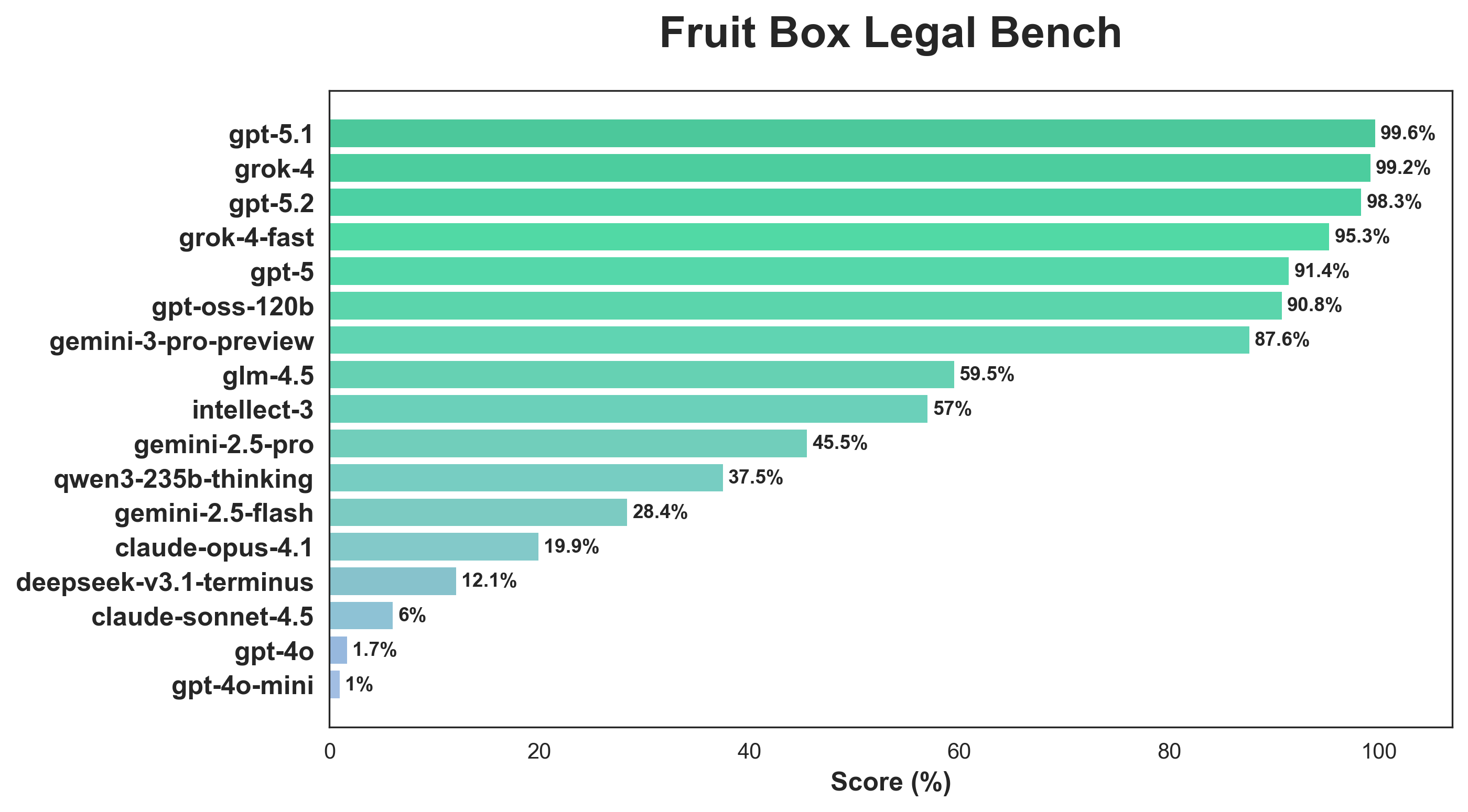
The gpt-5 and grok-4 families perform well, with gpt-5.1 and grok-4 achieving near-perfect accuracy on most rollouts. Interestingly, qwen3-235b-thinking, which achieved the second-highest score on the Fruit Box Bench, achieved only 37.5% on Fruit Box Start Legal Bench, suggesting its strength lies in strategic reasoning rather than exhaustive enumeration. Similarly, claude-sonnet-4.5 drops from 55.7% to 6.0%, indicating reliance on heuristic pattern matching rather than systematic verification. So in a sense, game-playing performance and systematic enumeration are distinct capabilities.
Prime Intellect’s intellect-3, post-trained on top of glm-4.5, improved on Fruit Box Bench and achieved roughly the same score on Fruit Box Start Legal Bench, though both still fall short of gpt-oss-120b, a model of comparable size. This gap likely stems from architectural and training differences: intellect-3 was post-trained on glm-4.5-air via SFT+RL on math, code, and science environments whereas gpt-oss-120b was designed for deeper reasoning and included various optimizations like sliding window attention for longer context handling, which becomes important in multi-turn environments.
SFT and GRPO
LLMs are great, and it’s perhaps unsurprising that they would achieve comparable performance to expert policies. A slightly more interesting avenue to pursue is how a pure RL agent would perform; think Cartpole or GDM’s Atari agents. The RL pipeline is split in two: one with a modified GRPO implementation from scratch, and the other with SFT on expert trajectories, to encode domain expertise—specifically the minimal area strategy—directly in the reward function.
architecture
The core challenge in Fruit Box is the large action space. To make this more feasible we use a factorized action space, splitting action selection into two phases: anchor and extent. This also coincides with a more natural intuition of how humans might think about the problem (pick a starting point, then decide how far to extend).
- phase-0 (anchor selection). The policy selects an anchor (top-left) point
(r1, c1)from the 170 cells. Anchor selection uses PPO, and since the action space is fixed at 170, we can use standard on-policy RL with GAE (Generalized Advantage Estimation) for value bootstrapping. - phase-1 (extent selection). Given the anchor, the policy selects an extent (bottom-right) point
(r2, c2)where $r2 \geq r1$ and $c2 \geq c1$. The action space here is variable, e.g. if the anchor is(6, 7), there are $(10-6) \times (17-7) = 40$ possible extents. Extent selection uses GRPO (Generalized Reward Policy Optimization) due to its algorithmic design for variable action spaces, where each candidate is simulated for a given anchor (without env execution). Unlike PPO which requires a fixed action space, GRPO can handle the variable number of valid extents per anchor.
The policy network is a CNN that processes a 4-channel observation tensor:
- channel 0: Normalized cell values (dividing by 9, 0-1 range)
- channel 1: Non-zero mask (1 where cells have values, 0 otherwise)
- channel 2: Anchor mask (all zeros in Phase-0, 1 at selected anchor in Phase-1)
- channel 3: Phase mask (all zeros in Phase-0, all ones in Phase-1)
The CNN architecture extracts spatial features via two convolutional layers (3x3 kernels, 32->64 channels with GroupNorm and GELU), flattens to a 256-dimensional feature vector, then branches into two heads: a policy head that outputs logits over actions, and a value head that estimates expected returns. The extent is mapped to be relative to the anchor, not the absolute position. The training was implemented in main forms of post-training:
-
pure RL: a modified GRPO from scratch, the policy initially learns via curriculum learning with sigmoid annealing that gradually exposes illegal actions to help the agent learn valid moves.
-
SFT (supervised fine-tuning): Next, I perform SFT on trajectories from expert policies (across the 4 policies). The SFT training treats each step as a classification problem, i.e. given the grid state and phase, predict the expert’s action.
All training was done on a variety of GPUs hosted by Prime Intellect, mostly H100s but also H200s and B200s. Many thanks to Johannes, Christian, and the rest of the Prime team for providing compute credits. For reproducibility, all training runs, hyperparameters, and model artifacts are logged on Weights & Biases for GRPO and SFT. It also includes (very informal) reports where you can look through the graphs and logs more carefully.
the learning problem: purity vs pragmatism
There’s a purist approach, and then there’s a pragmatic approach. In the latter, we simplify the learning problem by applying a legal mask so that the policy chooses only among legal moves. In this way, the policy only cares about learning a strategy (e.g. minimal vs greedy).
I happen to tend more on the “purist side,” which naturally involves many more problems. In this archetype, we need to consider
- learning the legality constraint: by adding a sum head to our CNN and pre-training to learn to minimize the mean absolute error between 10 and the sum of digits inside. However, determining the digits inside is a problem of phase-0 and phase-1 selection, so we run into the next problem:
- two-phase factorized action space: as mentioned before, the action space is factorized into phase-0 and phase-1. Treating them together can be computationally intractable, but factorizing it also separates two inherently related tasks; predicting the bottom-right corner means nothing without predicting the top-left corner first due to conditionality.
- an overdetermined loss stack: for each batch, we have cross-entropy on the positive action and a custom negative loss based on sampled illegal actions and masses for set-based losses. However, this leads to some contradictory gradient signals, like $p(expert)=1$, spreading the legal mass across all legal actions (so it doesn’t just learn the exact trajectory from the scripted policies), punishing exploration into illegal modes, etc. This can make the policy extremely conservative due to focusing on legality instead of exploration.
As we’ll see, this will later prove to be a hard learning problem, but I explore both the purist and the pragmatic approach.
RL results
All runs used 16 parallel environments, 128 rollouts per step, and a batch size of 512, as well as the same GRPO, GAE, and learning rate hyperparameters.
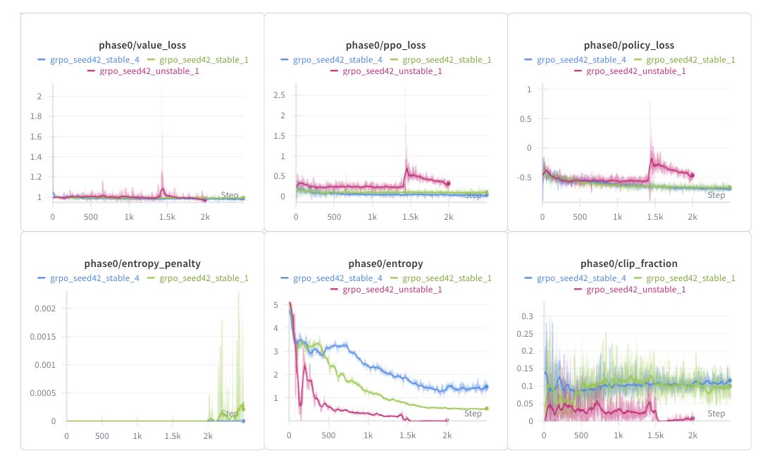
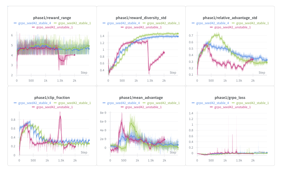
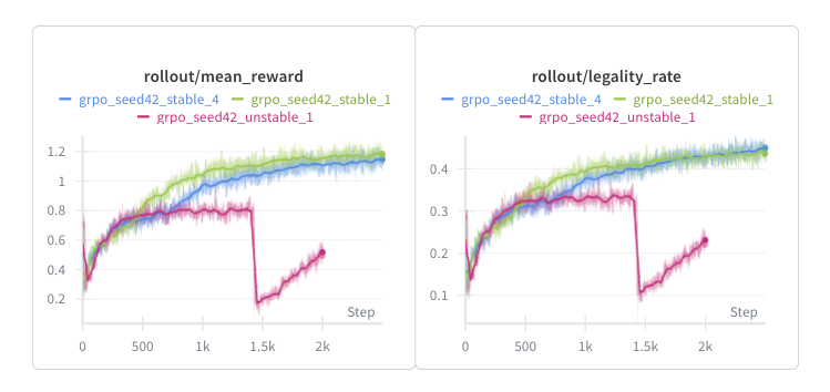
The initial GRPO run (grpo_seed42_unstable_1) looked promising for the first ~1k steps as the total reward and legality climbed gradually. But around step 1.4k, performance dropped significantly (-75% total reward, -70% legality rate), coinciding with spikes in the value, PPO, and policy loss for anchor selection as well as a drop in reward diversity std, indicating a collapse due to policy overconfidence. To fix this, we add various constraints related to entropy: increase the entropy coefficient and add an entropy target of 0.5. We also penalize illegal moves more (from -0.02 to -0.1) while making other minor changes to preserve the stability of the run.
The output (in green) is the first stable run, resulting in a legality rate of 0.43 and a mean reward of 1.2, therefore an average reward of $\frac{1.2}{0.43}=2.79$ per legal turn, considerably high and indicative of a greedy approach (rollouts were mostly based on starting moves, so the average is larger than the 2.6 mean reward of the greedy policy). However, the policy appears to be overfitting to high-reward patterns without learning the constraint that rectangles must sum to exactly 10. This is a common failure mode in RL when the reward signal is sparse and the constraint space is large.
To further improve learning, we tweak the CNN policy slightly by adding layernorm after the FC layers to normalize activations for gradient flow, and swap the ReLU for GeLU for smoother gradients. We also make small changes to entropy to maintain diversity throughout.
The output (in blue) is largely the same but with the entropy declining slower, and the reward accumulating slower. However, with a legality rate of 0.45 and a mean reward of 1.15, the policy achieves a much more reasonable reward of $\frac{1.15}{0.45}=2.56$ per legal turn, below the greedy policy. This run seems to have converged more slowly (entropy had not yet reached the entropy target); if the run had been extended by ~500-1k steps or the learning rate increased slightly, both the mean reward and legality rate would have likely exceeded that of the blue. This policy scores roughly between 70-90, which is not bad but still ~30 points below the minimal_area policy. With the large action space and sparse reward signal, this motivates using SFT to learn optimal strategies.
purist SFT results
We first consider a more pragmatic (but not fully rigorous) approach. For data, we have 2 choices:
- reuse the synthetic data generated via scripted policies (170k rows, 340k datapoints for both anchor and extent selection), so the SFT policy is able to learn from diverse strategies
- derive a minimal-area specific dataset to imitate the best policy.
We ended up choosing the latter to optimize for performance.
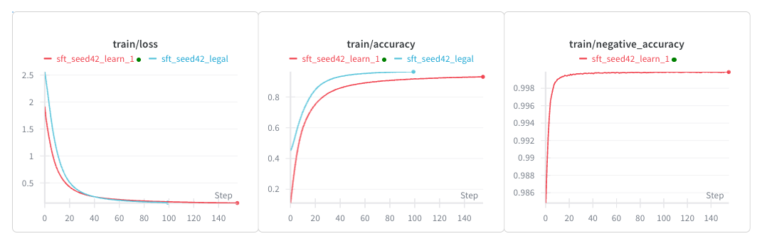
We first consider restricting the anchor and extent of the SFT policy to legal moves only (sft_seed42_legal). Of course, it learns quickly and achieves a 100% legality rate across multiple different initial grid configurations. Its results are most comparable to greedy, with an average of ~100 and max of ~135. This is probably due to the 2-step lookahead policy being essentially greedy (lookahead hardly matters until the late-stage, so for the vast majority of turns, lookahead and greedy give similar results). Importantly, because greedy is sub-optimal, we’ll perform more rigorous SFT that takes into account turn number to help motivate learning a strategy like minimal area. But this provides a comparable baseline for a pragmatic strategy.
Here, we switch gears into the more purist strategy. There are a few ideas (prefaced earlier in the learning problem section) that we bring to try to improve learning:
-
sum prediction head: we add an auxiliary head that predicts the sum of digits within each rectangle. This head is decoupled from the Phase-1 policy head to avoid gradient interference—the policy head learns which extent to select, while the sum head learns what the sum constraint means. When trained, the policy is frozen except for the feature extractors and the head itself.
-
anchor embedding: phase-1 extent selection is explicitly conditioned on the selected anchor via a learned 64-dimensional embedding. This models the dependency: choosing extent (r2, c2) depends on which anchor (r1, c1) was selected. We then concatenate the 256-dim feature vector (from the CNN) with the 64-dim anchor embedding to form the phase-1 head, giving it explicit access to anchor information rather than relying on implicit spatial reasoning.
-
pareto frontier hard negative mining: not all illegal actions are equally informative; for example, a relative extent of $(4,8)$ will rarely work (and only in the end-game) whereas a relative extent of $(1,2)$ is much more common. Suppose $(dr, dc)$ is the set of all valid extents for a given anchor which represents a sort of pareto frontier. We can mine hard negatives by considering the actions directly around the pareto frontier, since $(dr-1,dc)$ and $(dr, dc-1)$ must undershoot the sum while $(dr+1,dc)$ and $(dr,dc+1)$ must overshoot it (assuming no 0’s present).
- We use a 2:1 invalid/valid move ratio. Realistically, there are usually at most 200 valid moves (already generous) at a time, meaning the invalid-to-valid ratio is more like 41-to-1 instead of 1-to-1. But positive examples are more informative,
negative_loss_weightalready emphasizes negatives, and too many negatives can make the model overly conservative. We also log negative accuracy.
- We use a 2:1 invalid/valid move ratio. Realistically, there are usually at most 200 valid moves (already generous) at a time, meaning the invalid-to-valid ratio is more like 41-to-1 instead of 1-to-1. But positive examples are more informative,
-
set-based illegal mass losses: we penalize the model for placing probability mass on any illegal action simultaneously which helps to provide a stronger learning signal. It has 3 components that serve different purposes
4a. Illegal Mass Loss: $L_{\text{illegal}} = \alpha \cdot \sum p_{\text{illegal}} + \beta \cdot (\sum p_{\text{illegal}})^2$: a linear term to penalize total illegal probability, and a squared term to provide stronger gradient when illegal mass is high
4b. Top-K Illegal Loss: $L_{\text{topk}} = \delta \cdot \sum_{k=1}^{K} -\log(1 - p_{\text{illegal}_k})$: penalize the top-10 illegal actions by probability, and the logarithm for extra penalization for high-probability illegal actions
4c. Legal Mass Bonus: $L_{\text{legal}} = -\zeta \cdot \log(\sum p_{\text{legal}} + \epsilon)$: reward high probability mass on legal actions
-
multi-stage curriculum learning: there are 4 stages of curriculum learning
- a legal-only mask to build a foundation (even if the sum prediction head was trained)
- gradual curriculum exposure from a legal-only mask to all valid moves
- extent-size curriculum (from 4 to the max of 16) to roughly learn the minimal area strategy early
- turn-based curriculum to also incentivize the policy to learn the minimal policy by choosing smaller extents earlier
-
regularization: dropout ($p=0.1$), weight-decay (1e-4), and gradient clipping ($7.0$)
As a side note, although we did try separate pre-training for the sum prediction head, the initial few epochs for the non-pretrained and the pretrained runs were pretty identical, suggesting that the head is either architecturally insignificant or overfitted on training data. And while the 6 additions aren’t listed chronologically, each was motivated to improve learning further upon a previous run. The best run, using all six techniques, learned but not sufficiently:
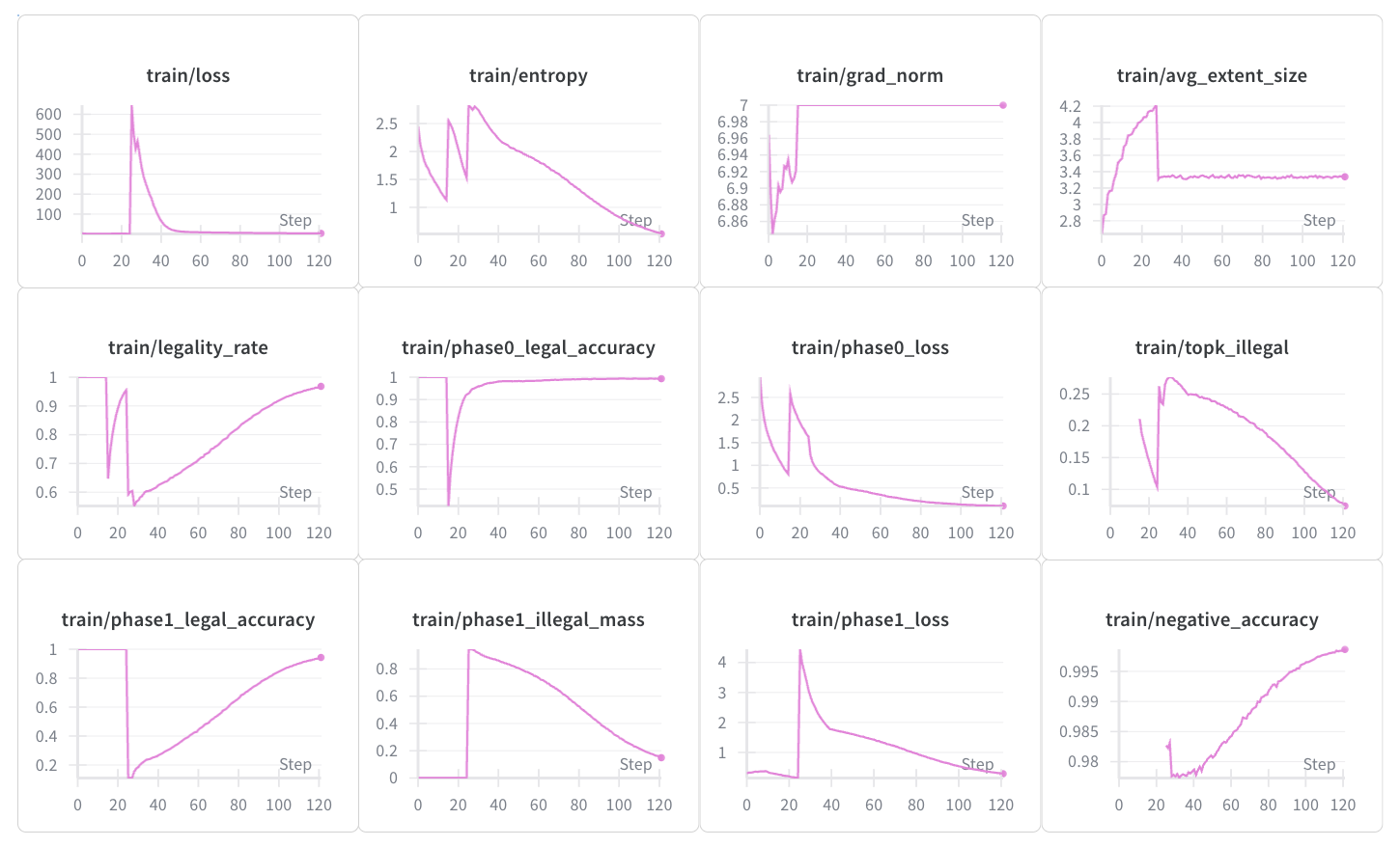
There are a few worrying signs of training here: the large grad_norm indicates large updates were still being made, and the monotonic increase in legality shows signs of overfitting. Tested on the training dataset over 50 grids with the following evaluation setup: ending on an illegal turn and allowing multiple tries (top-3 anchors × top-3 extents per turn), the policy achieves a mean legality rate of 92% but with an average score of 21.22 and max of 72. On random, unseen grids, the policy can correctly make the first move (94%), but proceeds to fail afterwards.
All is not lost! With the legal mask, the policy achieves an average of 107.3, beating all scripted policies by at least 5 points, except for minimal area (113.72); the SFT policy is only ~6 points below the expert minimal policy. This performance gap is surprisingly small given the complexity of learning both legality constraints and strategic play simultaneously.
The policy appears to have learned a hybrid strategy that balances immediate reward with some strategic preservation, though it hasn’t fully internalized the minimal area principle. When evaluated with legal masks (removing the burden of learning legality), the policy demonstrates clear strategic understanding: it consistently solves grids, achieves high completion rates (100% of grids solved within 60 moves), and clears an average of 107.33 cells per grid. The fact that it performs comparably to the minimal policy suggests it has learned some form of delayed gratification, even if not perfectly.
However, there are clear limitations. Looking at example trajectories, the policy is occasionally aggressive at the start, choosing larger rectangles early when smaller ones would preserve more options:
==============
Move 1 - Action: (0,1) -> (2,1) | Reward: 3 cells cleared
==============
    0  1  2  3  4  5  6  7  8  9 10 11 12 13 14 15 16
 0  6 [7] 9  7  5  7  2  3  8  7  9  8  1  1  1  3  8
 1  1 [2] 2  5  2  2  8  1  9  5  6  7  1  2  7  1  5
 2  6 [1] 4  7  2  4  3  6  9  8  2  3  2  3  6  9  3
 3  6  2  7  2  6  4  5  6  2  7  8  8  2  2  6  6  3
 4  5  7  7  9  1  6  1  9  1  9  8  6  7  7  9  1  5
 5  3  6  7  2  9  1  8  9  9  8  7  5  7  8  1  8  6
 6  3  7  4  2  4  7  5  1  2  2  2  3  5  4  1  4  1
 7  3  5  1  1  4  9  8  4  7  4  5  1  3  5  7  7  9
 8  4  2  7  7  6  3  1  7  2  3  7  8  7  6  1  2  7
 9  7  7  4  2  7  1  1  7  7  4  8  1  3  4  3  4  1

Selected rectangle: Sum = 10, Cells = 3, Reward = 3

==============
Move 2 - Action: (0,11) -> (0,13) | Reward: 3 cells cleared
==============
    0  1  2  3  4  5  6  7  8  9 10 11 12 13 14 15 16
 0  6  .  9  7  5  7  2  3  8  7  9 [8][1][1] 1  3  8
 1  1  .  2  5  2  2  8  1  9  5  6  7  1  2  7  1  5
 2  6  .  4  7  2  4  3  6  9  8  2  3  2  3  6  9  3
 3  6  2  7  2  6  4  5  6  2  7  8  8  2  2  6  6  3
 4  5  7  7  9  1  6  1  9  1  9  8  6  7  7  9  1  5
 5  3  6  7  2  9  1  8  9  9  8  7  5  7  8  1  8  6
 6  3  7  4  2  4  7  5  1  2  2  2  3  5  4  1  4  1
 7  3  5  1  1  4  9  8  4  7  4  5  1  3  5  7  7  9
 8  4  2  7  7  6  3  1  7  2  3  7  8  7  6  1  2  7
 9  7  7  4  2  7  1  1  7  7  4  8  1  3  4  3  4  1
Synthesizing all results now,
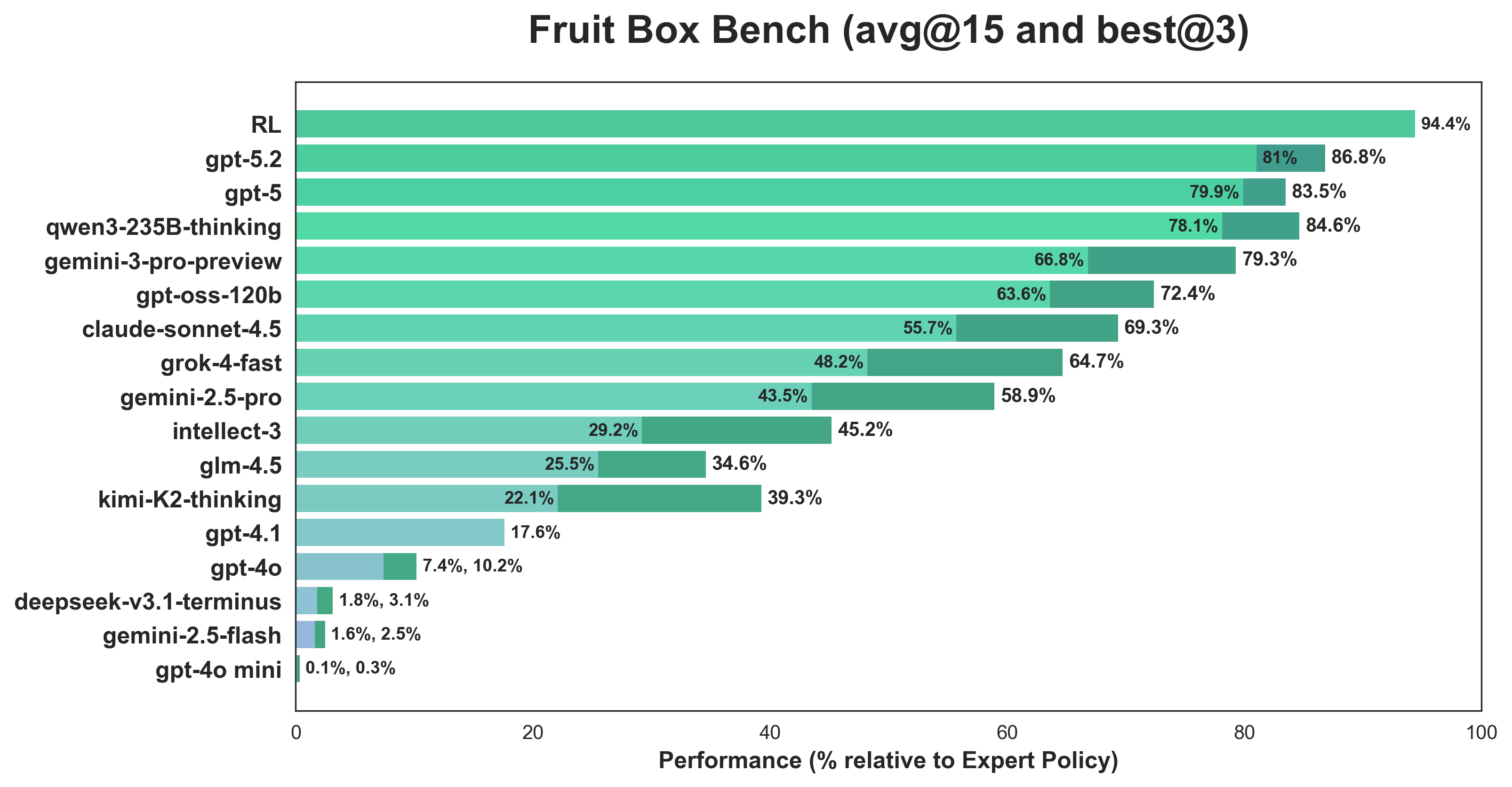
The RL agent (94.4%) outperforms all LLMs by a significant margin, even when considering best@3. This isn’t entirely unsurprising: we’d expect a specialized RL agent to outperform general-purpose reasoning LLMs. The RL agent processes the grid state directly through convolutional layers and learns spatial patterns while LLMs reason through text-based reasoning and convert that into spatial understanding. But, the fact that LLMs achieve 80%+ performance suggests they can reason spatially, just not as precisely. The 10-point gap likely reflects two limitations: first, LLMs struggle with the fine-grained pattern matching required for optimal play (e.g., recognizing when a 1-1-8 pattern is preferable to 2-8); second, their reasoning is inherently sequential and text-based, making it harder to maintain a global view of the board state across many turns.
I think there may be a ceiling imposed by the text-to-spatial translation overhead. LLMs likely encode some spatial understanding implicitly through their learned representations (attention patterns that track relative positions, embeddings that capture geometric relationships), but this encoding is indirect and may lose precision compared to architectures designed for spatial data.
Next Steps
While the current SFT results are promising, there are a few directions that I’d be excited to continue exploring:
-
Turn-Aware Features: Adding turn index information to the policy network could help it learn turn-dependent strategies (e.g., prefer smaller rectangles early). One idea is to use a learned turn embedding that gets added to the feature vector, which also preserves the pretrained CNN while allowing the policy to condition on game progress.
-
Return-Aware Objective: Weight examples by cumulative return using advantage-weighted loss: $w = \exp(\beta \cdot (G_t - \text{baseline}))$, naturally encoding the minimal area strategy without explicit curriculum design.
-
Explicit Pattern Training: Creating a library of “low-tech” patterns (like those mentioned at the beginning) and explicitly training on these patterns could help the policy learn local optimality. These could be specifically generated interspersing these low-tech patterns randomly on grids and having actions select the sequence of desired actions.
Beyond SFT-specific improvements, I’m also curious about a few other things:
-
VLM Evaluation: Testing VLMs with grid screenshots instead of LLMs could reveal whether direct visual processing improves spatial reasoning. VLMs might better capture spatial relationships, potentially closing the gap or beating RL agents and scripted policies.
-
Interpretability: Comparing RL and LLM reasoning could reveal complementary strengths. Attention patterns in LLM traces, CNN features, or human intuitions, decision boundary visualization could all reveal how different architectures approach spatial reasoning.