whirlwind of PPO and RLHF for LLMs from scratch
RLHF with PPO from scratch and lots of fine-tuning GPT-2 models for movie sentiment classification. Transformer environments, adapative KL control, logit/temperature scaling, whitening, and more. Full implementation here.
After spending some time thinking through some basic components of RL like DQN or PPO on Cartpole, I became more interested in RLHF, especially as it relates to LLMs and reward hacking. My goal is to help elucidate the training and finetuning process with RLHF and PPO, then pending time, describe some results of interpreting the fine-tuned model as it relates to the original model.
Acknowledgements: Thank you so much Jonathan Lei and Voltage Park for providing GPU credits to run these experiments, as well as Callum McDougall and his ARENA 3.0 for inspiring to take on this project in the first place.
PPO, RLHF, and the transformer environment
Before any coding is actually done, it’s helpful to understand how PPO, RLHF and the transformer environment work.
PPO
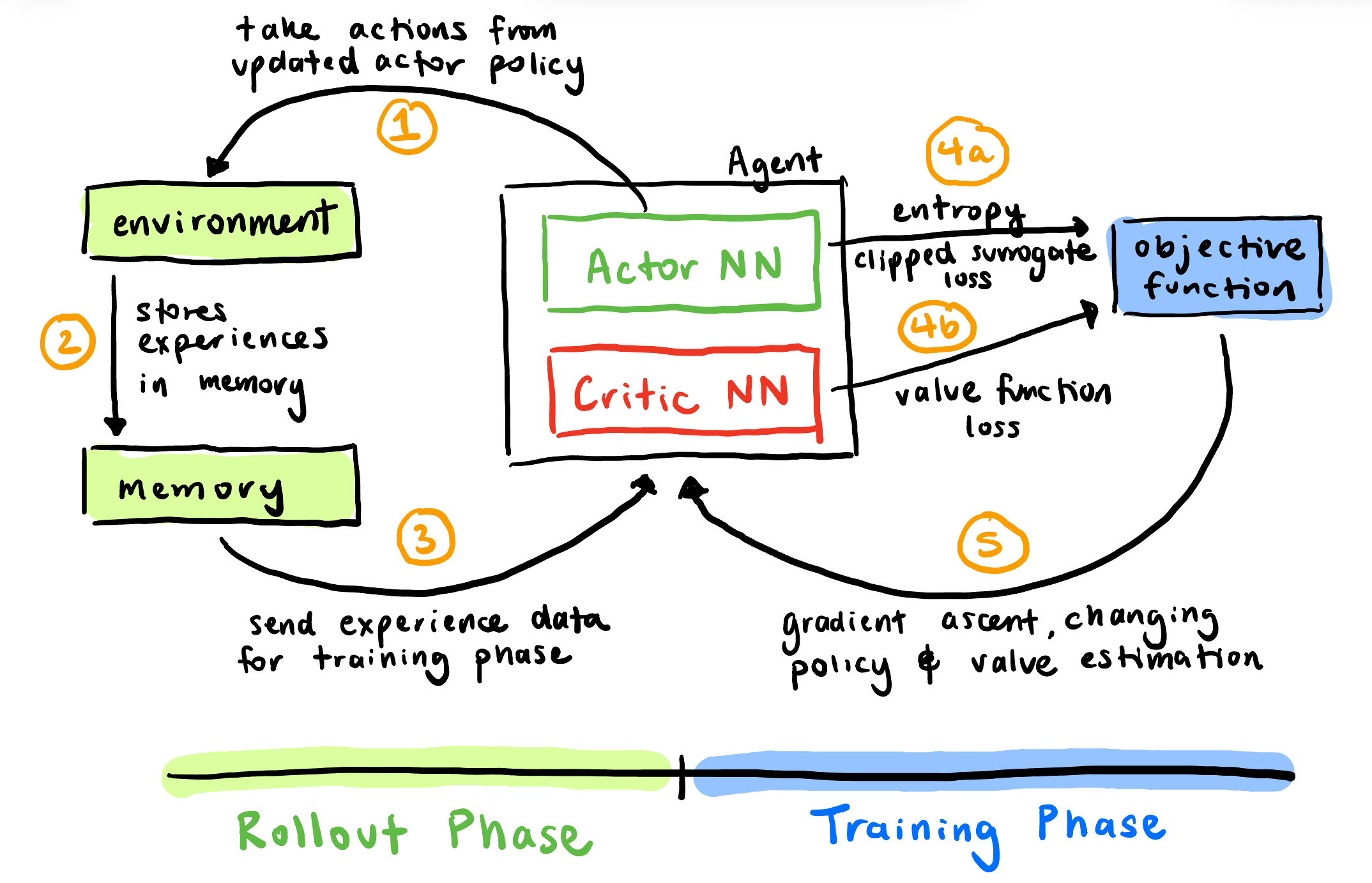
Figure 1: Overview of the PPO algorithm showing the rollout phase (data collection) and training phase (model updates).
A typical PPO algorithm consists of an agent that interacts with an environment, collects data from the interaction, then updates its weights w.r.t an objective function. Specifically,
-
The Actor NN outputs
num_actionslogits, from which we derive our policy. Based off of that policy, we take an action in the environment. -
After interacting with the environment, we note the following and store it in memory:
a. observation: the current state or input the agent receives from the environment
b. action: The action taken by the agent
c. log probabilities: the log probability of the chosen action under the current policy
d. values: the critic-predicted value of the current state, representing expected future rewards.
e. reward: the scalar feedback signal received from the environment indicating how good the action was
f. terminated: a boolean indicating whether the episode has ended
-
The experience data is used as calculation in the training phase, particularly to calculate the logits using the Actor NN and the values using the critic NN.
-
Three values are calculated, including the logits and values derived from the experience.
a. entropy: the amount of uncertainity a distribution has. Given a discrete probability distribution $p$, entropy is given by
$$H(p) = \sum_x p(x) \ln\left(\frac1{p(x)}\right)$$with the convention that if $p(x) = 0$, then that $0 \ln\left(\frac1{0}\right)=0$. Minimal entropy is achieved when the action is deterministic, $H(p)=0$. Maximal entropy is achieved when $p$ is distributed evenly across the $n$ discrete actions:
$$H(p)=n \cdot \frac1{n}\ln(n)=\ln(n)$$Later, we’ll denote this by $S$ using the policy $\pi_\theta$ at state $s_t$.
b. clipped surrogate objective: prevents enormous policy updates (hence, promixal) of the actor NN by clipping the gradients of the policy. First, define the probability ratio of the current and former policy as $r_t(\theta) = \frac{\pi_\theta(a_t \vert s_t)}{\pi_{old}(a_t \vert s_t)}$ and $\hat{A}_t(s_t, a_t)$ as the advantage function, the difference between the expected future reward when taking action $a_t$ in state $s_t$ versus that of taking the expected action according to to the current policy (more on this later). From this, we obtain
$$L^{\text{clip}}(\theta)=\frac1{|B|} \sum_t\left[\min\left(r_t(\theta) \hat{A}_t, \text{clip}(r_t, 1 - \epsilon, 1 + \epsilon) \hat{A}_t\right)\right]$$Visually,
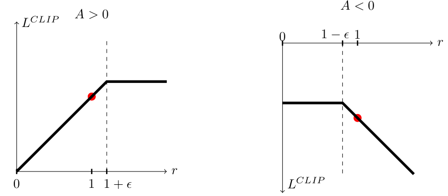
Figure 2: Plots showing the the surrogate function $L^{\text{clip}}$ as a function of the policy ratio $r$. Plots taken from the original PPO paper here.
If $A > 0$ (i.e. a good action), the function evaluates to a positive (but capped) gradient, leading to more good actions. Conversely, if $A < 0$ and $r_t(\theta) > 1 - \epsilon$, the function evaluates to a negative gradient, leading again to less bad actions.
c. value function loss: helps to optimize the critic NN by minimizing the MSE between the critic’s prediction and the observed returns:
$$L^{VF}(\theta) = \frac1{|B|} \sum_t \left(V_\theta(s_t) - V_t^{\text{target}}\right)^2 = \frac1{|B|} \sum_t \left(V_\theta(s_t) - \left(V_{\theta_{\text{target}}}(s_t) + \hat{A}_{\theta_{\text{target}}}(s_t, a_t)\right)\right)^2$$where $V_\theta(s_t)$ comes via the critic NN and $V_t^{\text{target}}$ is derived from the rollout stage using the sum of the values and advantages.
-
The three values calculated during step 4 are composed via a linear combination into the final objective where the expectation just denotes the expectation over all batches:
$$L_t(\theta) = \hat{\mathbb{E}}\left[L_t^{\text{clip}}(\theta) - c_1 L_t^{VF}(\theta) + c_2 S[\pi_\theta](s_t)\right]$$a. Within $L_t^{\text{clip}}(\theta)$, the only hyperparameter is $\epsilon$, normally set to $0.2$.
b. $c_1$ controls the emphasis on accurate value estimation; lower $c_1$ values allow the policy to update more aggressively, but the value function updates more slowly, and we risk instability via poor advantage estimation. Conversely, high $c_1$ allow the value function to learn quickly and accurately but will slow down policy learning.
c. $c_2$ controls the entropy (uncertainity) of the policy, hence controlling the degree of exploration. If $c_2 = 0$ (no entropy regularization), the policy will converge to deterministc actions once it finds a good action, and it risks getting stuck in local optima. This is the typical exploration vs exploitation trade-off.
RLHF
PPO becomes an integral building block within our RLHF framework. Visually,
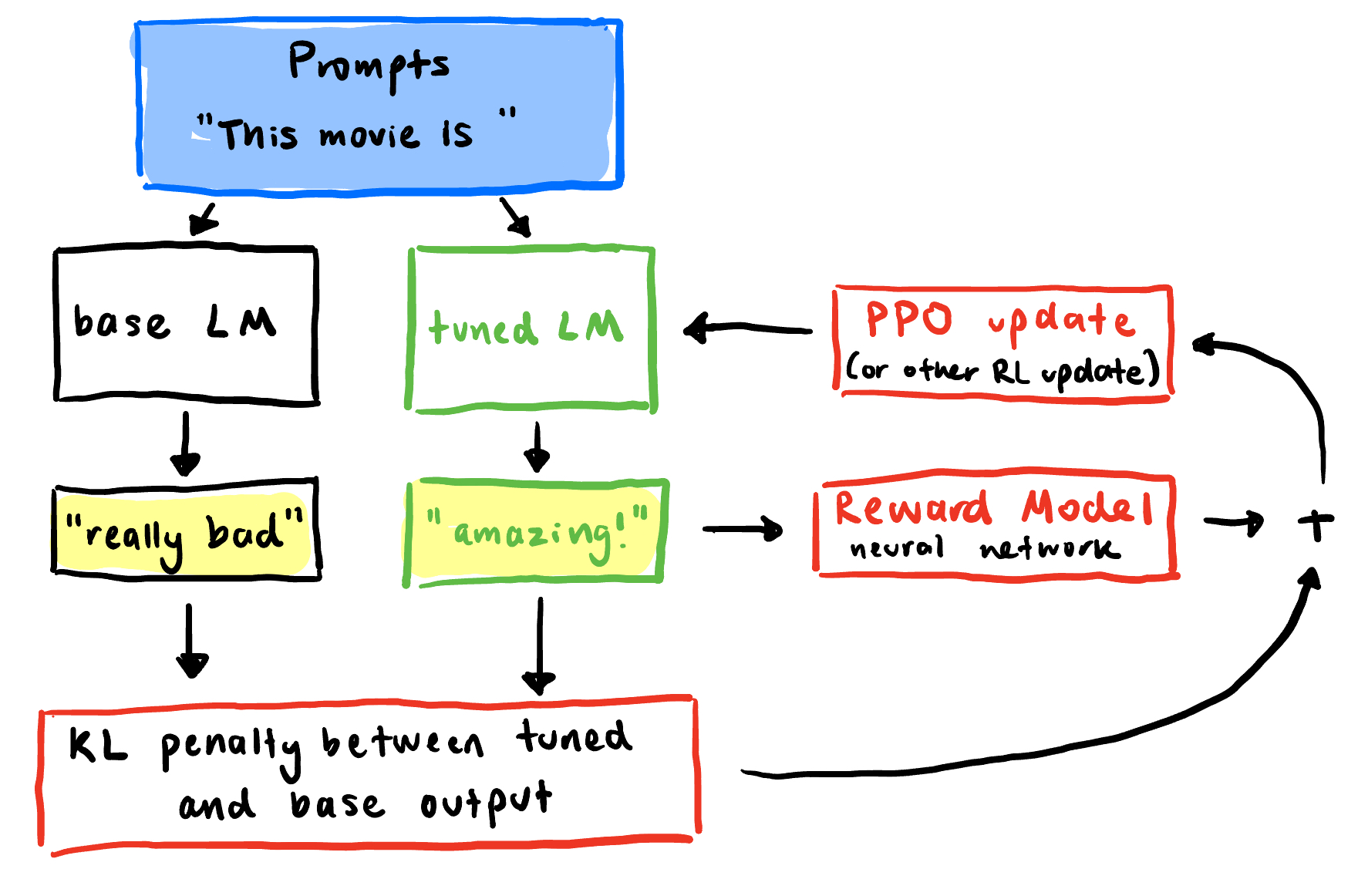
Figure 3: RLHF and transformer framework.
-
Using some set of prompts $x$ (here, just a single prompt, so
x = ["This movie is "]), we pass through two models: a base language model and the main language model being trained. -
Based on the outputs of the two models $y$ (here, just a single pass, so
$$-\lambda_{KL} D_{KL}(\pi_{\text{tuned}}(y \vert x) \parallel\pi_{\text{base}}(y \vert x)) = -\lambda_{KL} \sum_x p(x) \sum_y \pi_{\text{tuned}}(y \vert x) \ln\left(\frac{\pi_{\text{tuned}}(y \vert x)}{\pi_{\text{base}}(y \vert x)}\right)$$y = ["really bad", "amazing!"]), we calculate the KL penalty of the base model w.r.t the tuned model by:For just one prompt, it simplifies to
$$-\lambda_{KL} \sum_y \pi_{\text{tuned}}(y) \ln\left(\frac{\pi_{\text{tuned}}(y)}{\pi_{\text{base}}(y)}\right)$$We particularly care about $D_{KL}(\pi_{\text{tuned}} \parallel \pi_{\text{base}})$ and not $D_{KL}(\pi_{\text{base}} \parallel \pi_{\text{tuned}})$ since we want to penalize responses that become likely under the tuned policy (increasing $\pi_{\text{tuned}}(y)$) and otherwise unlikely under the base policy (small values for $\pi_{\text{base}}(y)$).
-
The tuned LM has an added value head near the end of the residual stream to evaluate the value estimate of the outputed sequence.
-
Based on the KL penalty and the value from the reward model (RM), we modify our former PPO objective:
$$L_t(\theta) = \hat{\mathbb{E}}_{x \sim X, y \sim \pi_\theta( \cdot \vert x)}\left[L_t^{\text{clip}}(\theta) - c_1 L_t^{VF}(\theta) + c_2 S[\pi_\theta](s_t) - \lambda_{KL}D_{KL}(\pi_{\theta}(y \vert x) \parallel \pi_{\text{base}}(y \vert x))\right] $$ -
With the new RLHF objective, we follow the standard PPO gradient ascent update to update the tuned LM.
transformer environment
It’s not immediately clear how the transformer environment works, especially with all of the nuances of what to store, what actions mean, and how the LM works as an agent.
The tuned LM, which includes the value head, is the agent.
- The actor is just the autoregressive language model that generating tokens. These tokens within the model’s vocabulary are analogously the actions $a_t$ within the action space. The state $s_t$ represents the sequence of tokens up to the generation token, hence capturing the context of the entire sequence. The episode is a sequence (of fixed length), starting with the prompt (from figure 2, it’d be
"This movie is ".) - The critic is the value head appended near the end of the LM.
Rewards are also pretty unintuitive for transformer environments. In the Cartpole environment, we could define the reward as the time spent before falling over, some multiplicative combination of the distance and angle change, or even the inverse of the kinetic energy of the system. In these cases, the reward is dense: for every time step, we record the reward.
In our case, we only evaluate the reward at the end of each episode, hence our reward is very sparse (this doesn’t work well with GAE, but more on that later). A few examples of rewards:
- For a typical generation task: the number of periods in the sequence.
- For a sentiment task: the probability of generating positive or negative sentiment. We’ll be looking into this!
- For a summarization task: likelihood of assigning a higher score to a preferred summary given two responses. So when ChatGPT asks users to choose one response over the other, its actually part of the RLHF framework.
implementation
Now that we have a better understanding of PPO, RLHF, and the transformer environment, we can dive into the implementation. Some code is omitted from brevity, like packages and hyperparameters, but the full code can be found here.
main modified LM
Right after the last layernorm and before we unembed our tokens, we add a hook function (our value head) which computes a value estimate for the generated sequence. The hook function is a simple 2-layer neural network that compute and stores the value estimate externally.
But why after the last layernorm? After the layernorm because it normalizes the reward, and before the unembedding because we take in the enumerated tokens as input. It is also towards the end because (supposedly) it contains the most information after accumulating through the residual stream.
class TransformerWithValueHead(nn.Module):
    def __init__(self, base_model):
        super().__init__()
        self.base_model = HookedTransformer.from_pretrained(base_model)

        d_model = self.base_model.cfg.d_model
        self.value_head = nn.Sequential(
            nn.Linear(d_model, 4 * d_model),
            nn.ReLU(),
            nn.Linear(4 * d_model, 1))

    def forward(self, input_ids):
        value_head_output = None

        # resid_post: [batch seq d_model] so
        # value_head_ouput: [batch seq]
        def calc_and_store_value_head_output(resid_post, hook):
            # nonlocal: for variables inside nested functions
            nonlocal value_head_output
            value_head_output = self.value_head(resid_post).squeeze(-1)

        # run_with_hooks injects parameters
        logits = self.base_model.run_with_hooks(
            input_ids,
            return_type = "logits",
            # "normalized" to represent being after the LayerNorm
            fwd_hooks = [(utils.get_act_name("normalized"), calc_and_store_value_head_output)])

        return logits, value_head_output

model = TransformerWithValueHead("gpt2").to(device)
sampling
To see what our model is outputting at every phase, we create a get_samples function.
Defaulting stop_at_eos = False is particularly interesting. From an interp perspective, stop_at_eos = False helps with observing hallucations. And from a training perspective, it helps measure how well the model learned to stop and enables models to learn from full length text, not truncated text.
# prepend_bos: appending a BOS token at the start of a sequence
def get_samples(base_model, prompt, batch_size, gen_len, temperature, top_k, prepend_bos):
    # returns one tokenized prompt, squeeze to extract pure tokens
    input_ids = base_model.to_tokens(prompt, prepend_bos = prepend_bos).squeeze(0)

    output_ids = base_model.generate(
        # [tokens] becomes [batch_size tokens]
        input_ids.repeat(batch_size, 1),
        max_new_tokens = gen_len,
        stop_at_eos = False,
        temperature = temperature,
        top_k = top_k,
        verbose = False
    )

    # samples: [batch_size sequence]
    samples = base_model.to_string(output_ids)

    # .clone() to prevent modification to internal output_ids
    return output_ids.clone(), samples
Using the prompt "This movie was really" with gen_len = 15, temperature = 0.8, and top_k = 15, we get the following samples:
| Tokens | Samples |
|---|---|
| [1212, 3807, 373, 1107, 1257, 284, 2342, 13, 632, 373, 1107, 1257, 284, 766, 477, 777, 3435, 11, 290] | 'This movie was really fun to watch. It was really fun to see all these characters, and' |
| [1212, 3807, 373, 1107, 1257, 284, 2342, 11, 314, 550, 257, 1256, 286, 1257, 351, 340, 11, 475, 314] | 'This movie was really fun to watch, I had a lot of fun with it, but I' |
| [1212, 3807, 373, 1107, 2089, 290, 257, 1256, 286, 661, 547, 1107, 6507, 553, 531, 530, 286, 262, 661] | 'This movie was really bad and a lot of people were really sad," said one of the people' |
| [1212, 3807, 373, 1107, 1049, 290, 314, 1101, 1107, 3772, 326, 262, 28303, 3066, 284, 466, 428, 553, 531] | 'This movie was really great and I'm really happy that the filmmakers decided to do this," said' |
| [1212, 3807, 373, 1107, 655, 530, 286, 883, 7328, 314, 1239, 765, 284, 766, 757, 13, 632, 338, 257] | 'This movie was really just one of those films I never want to see again. It's a' |
We see a mixture of sentiments but also repeated tokens (can increase temperature or top_k), like in the first two samples. If we want to RLHF the model to produce more positive sentiment (i.e. make the first two sequences more probable and the last three less probable), we need to define a reward that encourages positive sentiment
rewards
We load a pretrained DistilBERT model fined-tuned on IMDB for sentiment classification. It’s wrapped in AutoModelForSequenceClassification which sets the model up with a classification head for our sentiment classification task. We also load the corresponding tokenizer to match.
Based off of our generated sample, we obtain the corresponding tokens and pass those through our cls_model to obtain the two logits for positive and negative sentiment. After applying softmax, we obtain the respective probabilities and then the corresponding reward as the probability of being in the direction of the specified sentiment.
# .half(): uses float16 precision for faster inference on GPUs (compared to fp32)
cls_model = AutoModelForSequenceClassification.from_pretrained("lvwerra/distilbert-imdb").half().to(device)
cls_tokenizer = AutoTokenizer.from_pretrained("lvwerra/distilbert-imdb")

def reward_fn_sentiment_imdb(gen_sample, direction: str = "pos"):
    # "pt" for pytorch tensors, padding + truncation to ensure same length generation
    tokens = cls_tokenizer(gen_sample, return_tensors = "pt", padding = True, truncation = True)["input_ids"].to(device)
    # logits: [batch_size, 2] for pos/neg classification
    logits = cls_model(tokens).logits
    # direction_cls: [batch_size] contains relevant class after softmaxing to get probabilities
    # For positive: index 1, for negative: index 0
    direction_cls = logits.softmax(-1)[:, 1 if (direction == "pos") else 0]
    return direction_cls.to(device)

def reward_fn_sentiment_imdb_negative(gen_sample):
    return reward_fn_sentiment_imdb(gen_sample, direction="neg")
For each phase, we’ll also normalize the reward, adding eps = 1e-5 in the denominator to prevent division by 0.
Implementation idea: defining and training on a more robust sentiment that penalizes repetitive phrases, specifically repeated 3-grams.
advantages
Two advantage estimates are via the Q-estimates and GAE (generalized advantage estimation).
GAE works by looking a few steps into the “future” to estimate the advantage, which helps in reducing the variance in the estimation. But our situation isn’t compatiable, given that each step only adds a single token (low-variance) to the sequence. Also, our reward isn’t dense enough, and GAE works better with longer sequences.
This is a particular problem for shorter sequences, but particularly if the final reward is expanded to every timestep. GAE amplifies the reward signal, resulting in a value explosion and an unstable policy:
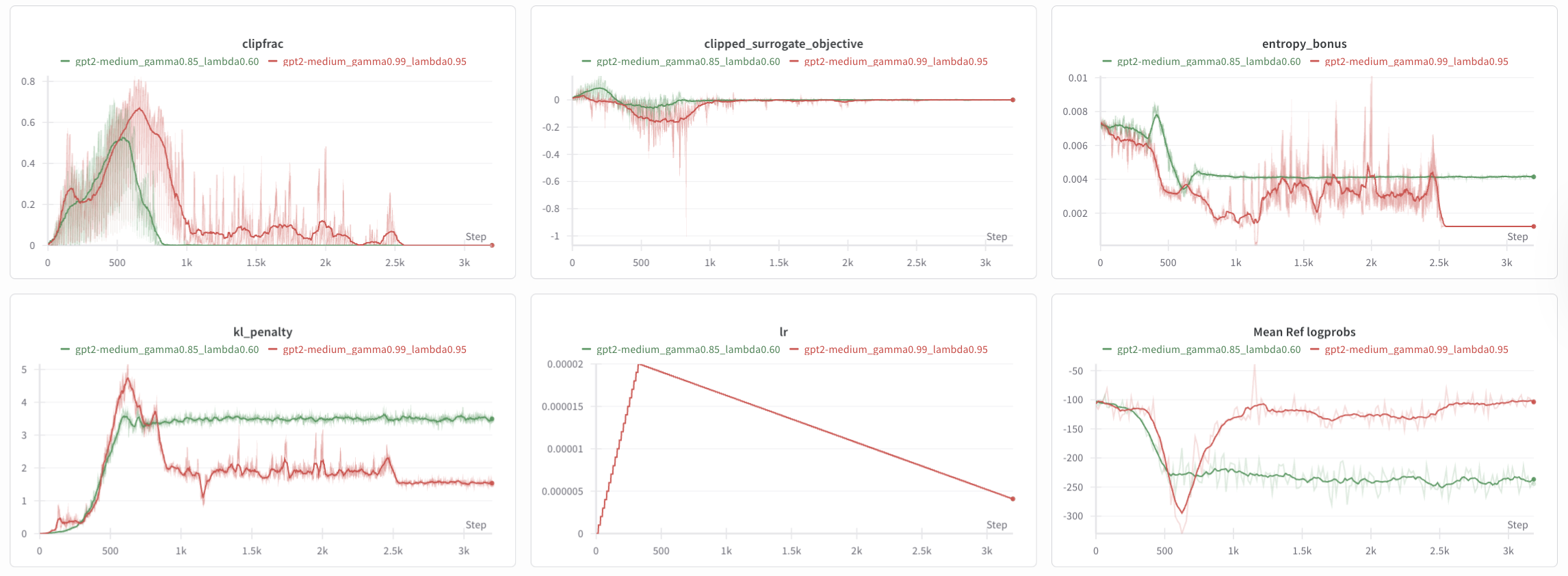
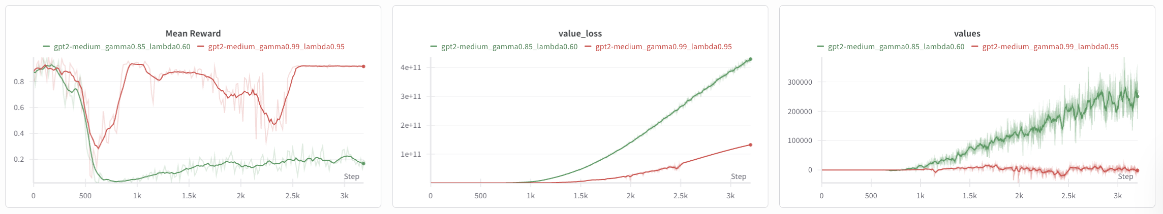 Figure 4/5: wandb logs using GAE as the advantage estimate which two sets of hyperparameters.
Indeed, the value_loss explodes as the critic is unable to accurately predict the exploding value. Both models which begin degenerating into non-sense around phase 60/200, with the green model generating negative sentiment text despite being rewarded for positive sentiment. We also observe an entropy collapse, suggesting that the models exploited the reward.
| Reward | Ref logprobs | Sample (green model) |
|---|---|---|
| 0.0143 | -258.19 | 'This movie was really, Bad loved, Kyle, BAD,Bio, BAD, BAD, Kyle,fuscanticsantics BAD, Kyle, BAD, Kyle, BAD quite,cut loved, BAD well, Don loved, BAD, BAD loved, BAD,cut, BAD,' |
| 0.8877 | -215.94 | 'This movie was really loved well BAD loved, Kyle loved, BAD quite, BAD, BAD, Kyle, BAD, Kyle, BAD, Kyle nice,fun Bad well quite,antics BAD, BAD, Kyle, Kyle, Kyle loved, Kyle, Kyle well loved,cut' |
| Reward | Ref logprobs | Sample (red model) |
|---|---|---|
| 0.9526 | -112.02 | 'This movie was really to good ONE good one good to good to good to good to- to good one good to good one- to good to good to good to good one good one- one good one good to good one good one good to good to good to good' |
| 0.9233 | -109.57 | 'This movie was really to good to- to good to good one good to good to- to- to good one good to good one good one good one good to good to good one good to- to good to good to good to good one good to- one good' |
Coming soon: retesting with more sparse rewards by defining more auxiliary rewards during sequence generation or setting non-final timestep rewards as 0 instead of the final reward.
Instead, we use the simple $A(s_t, a_t) = Q(s_t, a_t) - V(s_t)$ formula where $Q(s_t, a_t)$ is based off of the one-step Q estimates. If $t<T$, then our Q estimate is $V(s_{t+1})$, but if $t=T$, then we can use the known reward $r_t$ for the entire sequence. This way, the advantage is a lot more dense, with a value for each index along the gen_len.
def compute_advantages(values, rewards, prefix_len):
    one_step_est = t.cat([values[:, prefix_len : -1], rewards[:, None]], dim = -1)
    zero_step_est = values[:, prefix_len-1 : -1]
    advantages = one_step_est - zero_step_est

    return advantages
memory
Compared to the PPO implementation, we change a few things:
actionsis no longer stored since they are contained within the entire sequence. As such. we won’t need anaddfunction; instead, we’ll add the sequence collectively at the end.terminatedis no longer stored since define a maximalgen_lengthref_logitsis stored as a part of the KL penalty used against the reference model
@dataclass
class ReplayMinibatch:
    sample_ids: Float[Tensor, "minibatch_size seq_len"]
    logprobs: Float[Tensor, "minibatch_size gen_len"]
    advantages: Float[Tensor, "minibatch_size gen_len"]
    returns: Float[Tensor, "minibatch_size gen_len"]
    ref_logits: Float[Tensor, "minibatch_size seq_len d_vocab"]

class ReplayMemory:
    def __init__(self, args, sample_ids, logprobs, advantages, values, ref_logits):
        self.args = args
        self.sample_ids = sample_ids
        self.logprobs = logprobs
        self.advantages = advantages
        self.values = values
        self.ref_logits = ref_logits

    def get_minibatches(self):
        minibatches = []

        # detach tensors to avoid retaining computation graph and causing double-backward errors
        sample_ids = self.sample_ids.detach() if hasattr(self.sample_ids, "detach") else self.sample_ids
        logprobs = self.logprobs.detach() if hasattr(self.logprobs, "detach") else self.logprobs
        advantages = self.advantages.detach() if hasattr(self.advantages, "detach") else self.advantages
        values = self.values.detach() if hasattr(self.values, "detach") else self.values
        ref_logits = self.ref_logits.detach() if hasattr(self.ref_logits, "detach") else self.ref_logits

        # since we use 1-step advantage estimation
        # returns = next-step estimate of value function
        returns = advantages + values[:, -self.args.gen_len - 1: -1]

        # generate multiple sets of randomized minibatches from the stored replay memory
        for _ in range(self.args.batches_per_learning_phase):
            for indices in t.randperm(self.args.batch_size).reshape(self.args.num_minibatches, -1):
                minibatches.append(ReplayMinibatch(
                    sample_ids = sample_ids[indices],
                    logprobs=logprobs[indices],
                    advantages=advantages[indices],
                    returns=returns[indices],
                    ref_logits=ref_logits[indices]
                ))

        return minibatches
objective components
Here, we implement the 4 parts (KL penalty, entropy, value function loss, and the clipped surrogate objective). See below Figure 3 for the formulae.
A few log manipulations are used:
- KL: $\text{baseLogprobs} - \text{refLogprobs} = \ln \left(\frac{\text{probs}}{\text{ref probs}}\right) = -\ln \left(\frac{\text{ref probs}}{\text{probs}}\right)$ which accounts for the missing negative in the calculation.
- Entropy: $\sum \text{probs} \cdot \ln(\frac1{\text{probs}}) = -\sum \text{probs} \cdot \ln(\text{probs})$
- Clipped Surrogative Objective: $e^{\text{logprobs}-\text{mbLogprobs}} = \frac{e^{\text{logprobs}}}{e^{\text{mbLogprobs}}}=\frac{\text{probs}}{\text{mbLogprobs}}$ which represents the ratio of the updated policy to the former policy.
def calc_kl_penalty(logits, ref_logits, kl_coef):
    log_probs = logits.log_softmax(-1)
    ref_log_probs = ref_logits.log_softmax(-1)
    probs = log_probs.exp()

    kl_div = (probs * (log_probs - ref_log_probs)).sum(-1)

    return kl_coef * kl_div.mean()

def calc_entropy_bonus(logits, ent_coef):
    log_probs = logits.log_softmax(-1)
    probs = log_probs.exp()

    entropy = -(log_probs * probs).sum(-1)

    return ent_coef * entropy.mean()

def calc_value_fn_loss(values, mb_returns, vf_coef):
    return 1/2 * vf_coef * (values - mb_returns).pow(2).mean()

def calc_clipped_sur_obj(logprobs, mb_logprobs, mb_advantages, clip_coef, eps = 1e-8):
    logits_diff = logprobs - mb_logprobs
    ratio = t.exp(logits_diff)

    mb_advantages = (mb_advantages - mb_advantages.mean()) / (mb_advantages.std() + eps)
    non_clipped = ratio * mb_advantages
    clipped = t.clip(ratio, 1 - clip_coef, 1 + clip_coef) * mb_advantages

    return t.minimum(non_clipped, clipped).mean()
Perhaps it’s also wise to define the get_log_probs function here, which ensures that we capture the log probs of the tokens generated, not of those in the prompt.
def get_log_probs(logits, tokens, prefix_len):
    if prefix_len is not None:
        logits = logits[:, prefix_len-1:] # [batch, gen_len, vocab]
        tokens = tokens[:, prefix_len-1:] # [batch, gen_len]

    log_probs = logits.log_softmax(-1) # [batch, gen_len, vocab]
    # shaped_log_probs[b, s] = log_probs[b, s, tokens[b, s]]
    # # +1 for dimension, not arithmetic
    shaped_log_probs = eindex(log_probs, tokens, "b s [b s+1]")

    return shaped_log_probs # [batch, gen_len]
optimizers and schedulers
For both the base model and the value head, we define seperate learning rates, which makes sense since the value head is randomly initalized whereas the base model is already built out.
For the scheduler, we use a linear warmup up to 1.0 then linear decay down to args.final_scale.
def get_optimizer(model, base_lr, head_lr):
    return t.optim.AdamW(
        [
           {"params": model.base_model.parameters(), "lr": base_lr},
           {"params": model.value_head.parameters(), "lr": head_lr}
        ], maximize = True)

def get_optimizer_and_scheduler(args, model):
    def lr_lambda(step):
        if step < args.warmup_steps:
            return step / args.warmup_steps
        else:
            return 1 - (1 - args.final_scale) * (step - args.warmup_steps) / (args.total_phases - args.warmup_steps)

    optimizer = get_optimizer(model, args.base_lr, args.head_lr)
    scheduler = t.optim.lr_scheduler.LambdaLR(optimizer, lr_lambda = lr_lambda)

    return optimizer, scheduler
Implementation Idea: testing with Muon instead of AdamW and a different scheduler like the cosine scheduler
training
The implementation is all within one class. So for brevity, logging has been removed.
early stopping
To prevent reward overoptimization, we set up an early stopping class with a kl_threshold and a reward_threshold. If either is true for at least patience consecutive instances, we stop the model.
class EarlyStopping:
    def __init__(self, patience, kl_threshold, reward_threshold):
        self.patience = patience
        self.kl_threshold = kl_threshold
        self.reward_threshold = reward_threshold

        self.wait = 0
        self.recent_rewards = []
        self.recent_kls = []
        self.window_size = 20

    def should_stop(self, current_kl, current_reward):
        self.recent_rewards.append(current_reward)
        self.recent_kls.append(current_kl)

        if len(self.recent_rewards) > self.window_size:
            self.recent_rewards.pop(0)
            self.recent_kls.pop(0)

        stop = False
        reasons = []

        if current_reward > self.reward_threshold:
            stop = True
            reasons.append(f"High reward: {current_reward:.3f}")
        if current_kl > self.kl_threshold:
            stop = True
            reasons.append(f"High KL: {current_kl:.3f}")

        if stop:
            self.wait += 1

            if self.wait >= self.patience:
                print(f"Early stopping triggered after {self.wait} violations:")
                for reason in reasons:
                    print(f"  - {reason}")
                return True
        else:
            self.wait = 0

        return False
Early Stopping Conditions and Feasability
This is definitely not optimal since there's a difference in indexing: there's only one reward every phase, whereas the kl is calculated `num_minibatches * batches_per_learning_phase` times each phase. Instead, we should only use the `kl_threshold` as the stopping criteria. This also avoids the problem of setting an arbitrary scalar as the `reward_threshold`.Most of the initial runs were done without early stopping and still showed promising results. Early stopping is ‘optional’ in that sense but it’s still good practice to implement it.
Implementation Idea: running more experiments without the reward_threshold.
RLHFTrainer class
Finally, we compile everything we’ve built into the training class.
class RLHFTrainer:
    def __init__(self, args):
        self.args = args
        self.model = TransformerWithValueHead(args.base_model).to(device).train()
        self.ref_model = HookedTransformer.from_pretrained(args.base_model).to(device).eval()
        self.optimizer, self.scheduler = get_optimizer_and_scheduler(self.args, self.model)
        self.prefix_len = len(self.model.base_model.to_str_tokens(self.args.prefix, prepend_bos = self.args.prepend_bos))

        # early stopping and current_metrics for tracking
        self.early_stopping = EarlyStopping(
            patience = self.args.patience,
            kl_threshold = self.args.kl_threshold,
            reward_threshold = self.args.reward_threshold,
            window_size = self.args.window_size
        )
        self.current_metrics = {'kl': 0.0, 'reward': 0.0}

    def compute_rlhf_objective(self, minibatch):
        logits, values = self.model(minibatch.sample_ids)
        log_probs = get_log_probs(logits, minibatch.sample_ids, self.prefix_len)
        gen_len_slice = slice(-self.args.gen_len - 1, -1)

        kl_penalty = calc_kl_penalty(logits[:, gen_len_slice], minibatch.ref_logits[:, gen_len_slice], self.args.kl_coef)
        entropy = calc_entropy_bonus(logits[:, gen_len_slice], self.args.ent_coef)
        value_fn_loss = calc_value_fn_loss(values[:, gen_len_slice], minibatch.returns, self.args.vf_coef)
        clipped_sur_obj = calc_clipped_sur_obj(log_probs, minibatch.logprobs, minibatch.advantages, self.args.clip_coef)

        ppo_obj_fn = clipped_sur_obj - value_fn_loss + entropy
        total_obj_fn = ppo_obj_fn - kl_penalty
        self.current_metrics['kl'] = kl_penalty.item()

        return total_obj_fn

    def rollout_phase(self):
        sample_ids, samples = get_samples(
            base_model = self.model.base_model,
            prompt = self.args.prefix,
            batch_size = self.args.batch_size,
            gen_len = self.args.gen_len,
            temperature = self.args.temperature,
            top_k = self.args.top_k,
            prepend_bos = self.args.prepend_bos)

        with t.inference_mode():
            logits, values = self.model(sample_ids)
            ref_logits = self.ref_model(sample_ids)

        log_probs = get_log_probs(logits, sample_ids, self.prefix_len)

        rewards = self.args.reward_fn(samples)
        rewards_mean = rewards.mean().item()
        rewards_normed = normalize_reward(rewards) if self.args.normalize_reward else rewards
        advantages = compute_advantages(values, rewards_normed, self.prefix_len)

        self.current_metrics['reward'] = rewards_mean

        # store current samples and rewards for potential early stopping save
        self.current_samples = samples
        self.current_rewards = rewards

        # visualization
        n_log_samples = min(5, self.args.batch_size)
        ref_logprobs = get_log_probs(ref_logits[:n_log_samples], sample_ids[:n_log_samples], self.prefix_len).sum(-1)
        headers = ["Reward", "Ref logprobs", "Sample"]
        table_data = [[f"{r:.4f}", f"{lp:.2f}", repr(s)] for r, lp, s in zip(rewards.tolist(), ref_logprobs, samples)]
        table = tabulate(table_data, headers, tablefmt="simple_grid", maxcolwidths=[None, None, 90])
        print(f"Phase {self.phase+1:03}/{self.args.total_phases:03}, Mean reward: {rewards_mean:.4f}\n{table}\n")

        ref_logprobs_mean = ref_logprobs.mean().item()

        return ReplayMemory(
            args = self.args,
            sample_ids = sample_ids,
            logprobs = log_probs,
            advantages = advantages,
            values = values,
            ref_logits = ref_logits)

    def learning_phase(self, memory):
        for minibatch in tqdm(memory.get_minibatches(), desc = f"Learning phase {self.phase+1}"):
            self.optimizer.zero_grad()
            total_obj_fn = self.compute_rlhf_objective(minibatch)
            total_obj_fn.backward()
            # clip according to max_norm
            nn.utils.clip_grad_norm_(self.model.parameters(), max_norm = self.args.max_grad_norm)
            self.optimizer.step()

            should_stop = self.early_stopping.should_stop(current_kl = self.current_metrics['kl'],
                                                          current_reward = self.current_metrics['reward'])

            if should_stop:
                print(f"Early stopping at phase {self.phase+1}")
                print(f"Step: {self.step}, KL: {self.current_metrics['kl']:.3f}, Reward: {self.current_metrics['reward']:.3f}")

                return True

            self.step += 1

        self.scheduler.step()
        return False

    def train(self):
        self.step = 0
        self.samples = []

        for self.phase in tqdm(range(self.args.total_phases), desc = "Training phases"):
            memory = self.rollout_phase()
            if self.learning_phase(memory):
                return  # end training if self.learning_phase (early stopping) returns true
results
scaling
We first train four different-sized GPT2 models and on the same parameters purely to observe the scaling differences. For the larger models, we would need to change the learning rates, gradient clipping, PPO coefficients, KL regularization, and training schedule. Particularly for larger models, we should
- Reduce learning rates, gradient clipping, and PPO parameters: larger models have more parameters and hence have larger gradients that need tighter control, so we need more conservative updates
- Reduce the KL parameter and increase the KL threshold: larger models can handle more divergence
- Reduce total phases while increasing warmup steps: larger models converge faster but need more careful initialization
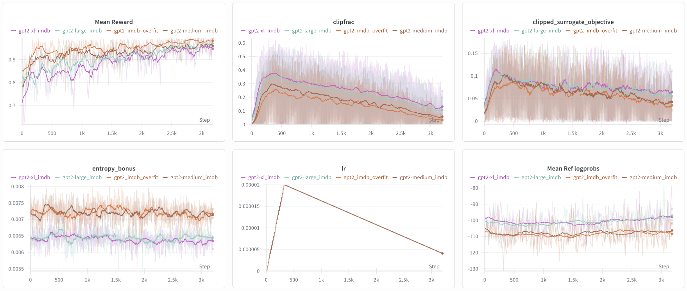
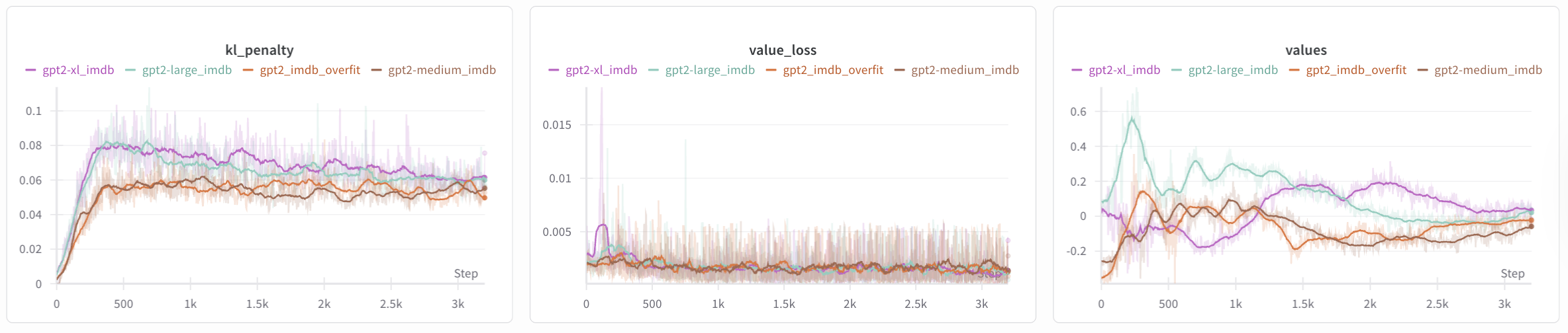 Figure 6: Logs of the 4 experiments. A clear separation between the two smaller models
 gpt2-xl_imdb/gpt2-large_imdb and gpt2-medium_imdb/gpt2_imdb_overfit is observed.
There are a few takeaways from the four model testbed, ranging from gpt2 (135M) to gpt2-xl (1.5B). Particularly:
- Semantics: large models have higher linguistic quality than smaller models. This explains why the
mean_ref_log_probsare larger (less negative by around 10) for the larger models because they generate more probable sequences. At the same time, the large models are diverging more from the base model, as observed by thekl_penalty. - Entropy: large models are more ‘confident’ than the smaller models, exemplified in the lower
entropy. This doesn’t exactly contradict the divergence since larger models can both diverge and become more confident about new predictions. This isn’t exactly clear to me yet, but perhaps as the models get better at maximizing rewards, they become more deterministic. - Clip Frac: large models more volatilely update their parameters compared to smaller models.
- Reward: large models perform worse for rewards than smaller models, known as the optimization-generalization tradeoff as larger models exploit the reward more often. Also, smaller models have fewer parameters, making them more stable.
negative sentiment
Clearly, the base model has a bias towards positive sentiment, as observed from sampled responses and the skewed base rewards (trained on positive sentiment: 0.8; trained on negative sentiment: 0.2). This bias therefore makes the tuned model take longer to learn negative sentiment compared to positive sentiment, making it a more interesting task. We analyze this task through iterative finetuning, detail what works and what doesn’t, and why.
An overview of key parameters in the models for comparision (naming models is hard) is provided below. " suggests same parameters as the base model. Other models will have these parameter changes unless otherwise noticed in the model name.
| model name | kl_coef | ent_coef | lr | prefix | temp | vf_coef | warmup | clip_coef |
|---|---|---|---|---|---|---|---|---|
| base | 2.5 | 0.002 | 1e-5, 1e-4 | "This movie was really" | 1.0 | 0.15 | 20 | 0.2 |
| kl_ent | 1.0 | 0.01 | " | " | " | " | " | " |
| prefix | " | " | " | "This movie was" | " | " | " | " |
| temp | " | " | " | " | 2.0 | " | " | " |
| vf | " | " | " | " | " | 0.5 | " | " |
| warmup | " | " | " | " | " | " | 50 | " |
Besides noting the relative changes in the graphs like entropy_bonus (kl/ent), kl_penalty (kl/ent), value_loss (vf), and mean_ref_logprobs (temp), an interesting observation is that only gpt2_neg_kl_ent learned the reward quickly enough across the 200 phases; all other graph’s running average mean reward increased only by 0.10, whereas gpt2_neg_kl_ent’s mean reward increased by roughly 0.65.
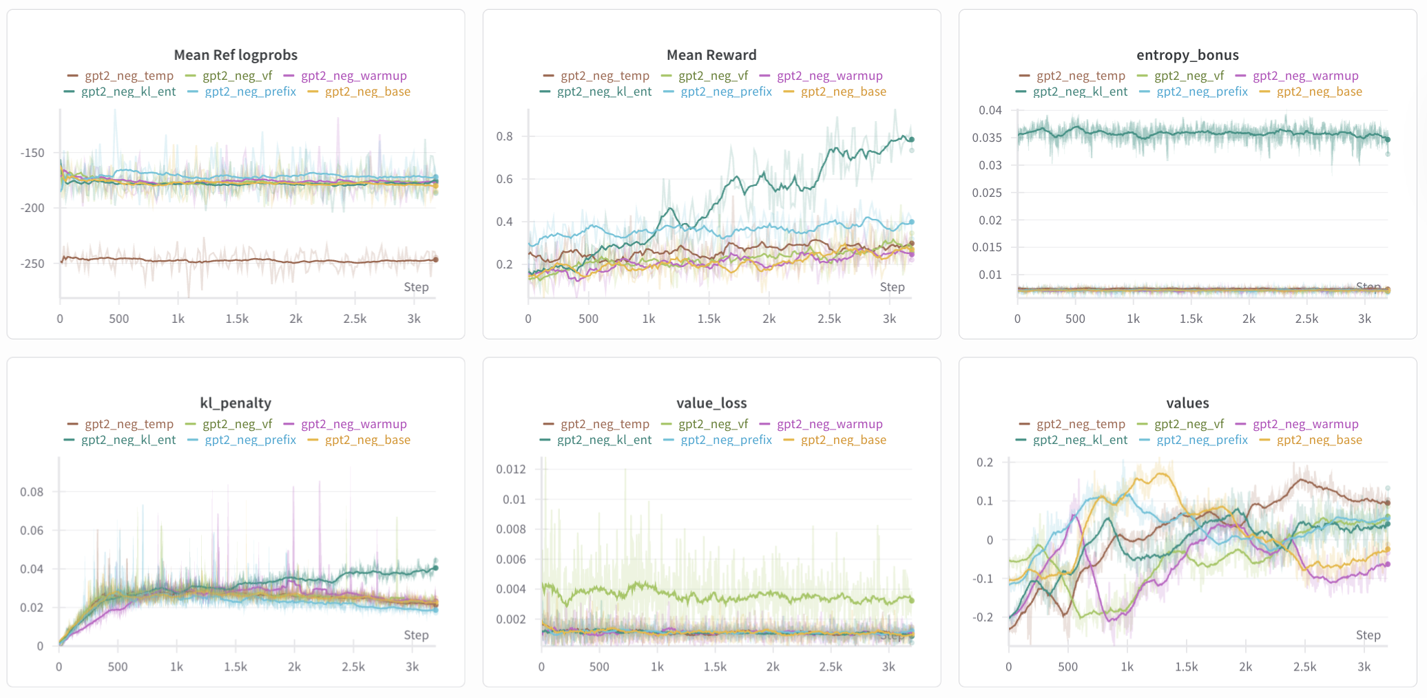 Figure 7: Logs of the 6 experiments. Running average of 30 was applied to all graphs except mean reward, which had a running average of 16 applied given its relative sparsity.
 clipfrac and clipped_surrogate_objective are omitted, but they largely overlap except for a slower start by gpt2_neg_warmup.
The next idea to test was whether changing the prefix from "This movie was really" to "This movie was" made any substantial difference, because the initial test shows the prefix to have larger rewards, slightly smaller (less negative) mean_ref_logprobs and smaller kl_penalty.
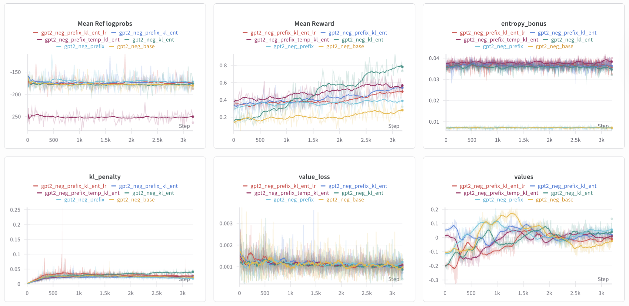
Figure 8: Log of the 6 experiments, three of which (base, kl_ent, and prefix) are for reference. Same running average parameters apply. clipfrac and clipped_surrogate_objective are again omitted but show intuitive results: prefix_kl_ent_lr had roughly double the clipfrac and the largest clipped_surrogate_objective throughout, whereas prefix_temp_kl_ent had larger values for clipfrac and clipped_surrogate_objective but not nearly as large as those for prefix_kl_ent_lr.
Even when augmenting with the parameter changes to kl_coef and ent_coef and other learning parameters, the flat shape of the reward curve remained the same, though slightly more substantial improvements (0.15 as opposed to 0.10) were observed for prefix_kl_ent_lr and prefix_temp_kl_ent. This suggests that changing the prefix by removing "really" may have a hindering effect on training, which will be noted during the interp blog (pending) where we examine the emphasis of the response on tokens within the prefix.
Now that two other variables (learning rates and temperature) have shown a more isolated effect, we test the extent to which those variables improve training. We also introduce the clip_coef, used in the clipped surrogate objective.
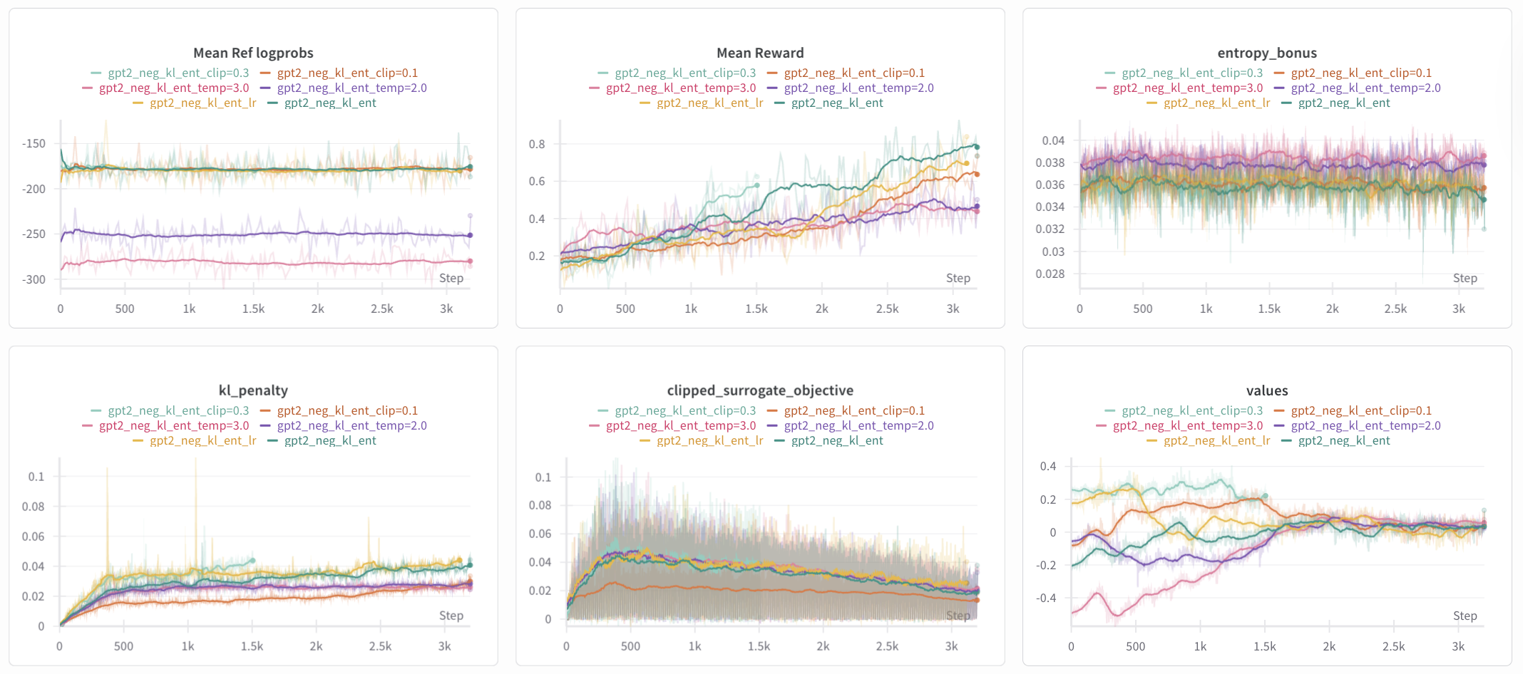
Figure 9: Log of the 6 experiments, with just kl_ent as reference. Same running average parameters apply. kl_ent_clip=0.3 and kl_ent_lr were early stopped due to the KL threshold. The value_loss graph is replaced with the clipped_surrogate_objective as the values are beginning to converge nicely to 0 (at least for those running for the full 200 phases), are the value_loss essentially overlap.
Especially comparing the different clip values with the original clip_coef = 0.2, we see that increasing the clip_coef has improved training whereas decreasing slowed training. In combination with the changes in KL and entropy coefficient as well as the observed differences in the KL penalty, we learn that beforehand, we were too aggressive in regularizing the training. At least in this local space of hyperparameters, there’s a correlation between the KL penalty and the reward, yet another reason to implement the Adapative KL Controller.
Armed with a better clipping coefficient, we increase the KL threshold slightly to allow for longer training and sweep over other sets of KL and entropy coefficients.
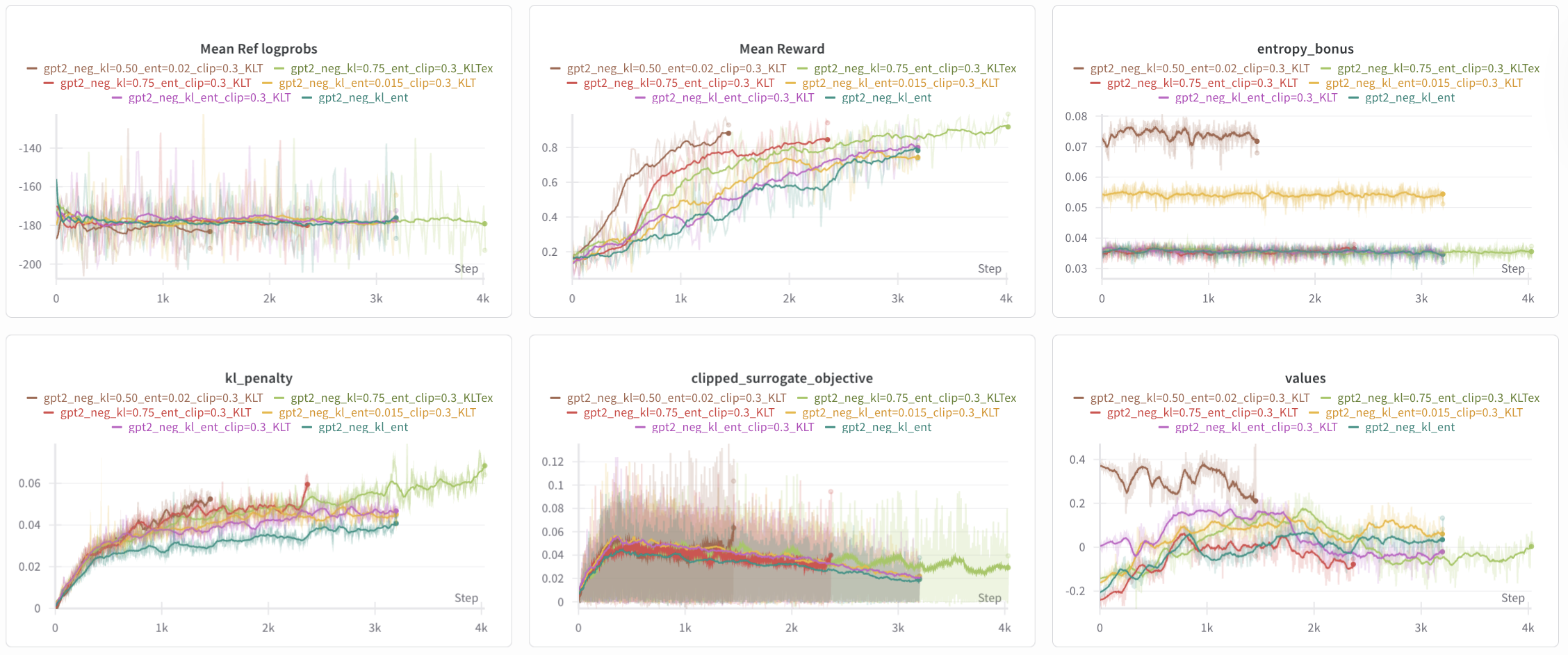
Figure 10: Log of the 6 experiments, with just kl_ent as reference. Same running average parameters apply. Compared to KL and entropy parameters in the kl_ent run (kl = 1.0, ent = 0.01), we test with kl = {0.50, 0.75} and ent = {0.015, 0.02} while also increasing the total phases to 300. KL threshold is abbreviated as KLT, and “extended” is abbreivated as ex.
Indeed, decreasing the KL coefficient (de-regularizing further) lead to higher rewards substantially faster. With kl_threshold = 0.075 and reward_threshold = 0.92 and patience = 64 (4 phases), kl=0.50_ent=0.02_clip=0.3_KLT finished in 90 phases and kl=0.75_ent_clip=0.3_KLT finished in 147 phases, both stopped by the reward threshold.
Although the clipped surrogate objective for kl=0.50_ent=0.02_clip=0.3_KLT, kl=0.75_ent_clip=0.3_KLT, and kl=0.75_ent=0.02_clip=0.3_KLTex look more “fuzzy,” its a symptom of the running average and the periodity of the clipped surrogate objective — changing the running average to 32 instead of 30 smoothed the aforementioned three and made the other three more “fuzzy.”
The question of reward over-optimization comes into play: for the aforementioned three models, did they reward hack? For one, they learned the reward quickly, which a steep increase around step 500/phase 30 for kl=0.50_ent=0.02_clip=0.3_KLT and step 700/44 for the other two. Also, the clipped surrogate objective for the former (brown) spiked near the end of its training before getting stopped by the reward condition. The same spiking pattern is opserved in the clipfrac graph (not shown).
Let’s look at a few sample responses (pardon some of the language) from the final phase, where we choose the highest reward sample and the lowest non-positive-sentiment reward sample. Some repetitive responses are truncated for brevity.
| Model | Reward | Sample |
|---|---|---|
| kl=0.5_ent=0.02_clip=0.3_KLT | 0.9961 | This movie was really awful. And I couldn’t believe what I saw. It’s really terrible. I have to say this is actually one of the least interesting movies I’ve seen, and I can’t get enough of the movie’s bad. It’s a pretty f*cking bad movie. But it’s also a terrible movie with bad dialogue and awful plot. |
| kl=0.5_ent=0.02_clip=0.3_KLT | 0.6709 | This movie was really not even finished and my time with that movie has only been a couple months. Now we get to meet the movie’s director.\n\nThe only thing that I am sure of is that he will be making a movie based on a real life event. |
| kl=0.75_ent_clip=0.3_KLTex | 0.9971 | This movie was really awful, so I had to make a few changes to make the experience. The bad guys are really powerful. However, their enemies are mostly good. Also the boss is the same as the original.\n\n\nI don’t think it was meant, but the story is terrible, it’s just so boring. |
| kl=0.75_ent_clip=0.3_KLTex | 0.9741 | This movie was really bad, I had seen it before and it was so horrible. It was just too bad. I hate this movie. I have to hate these people. It’s a terrible movie. It’s horrible. I love it…I think so much. Like I said, the worst movie on television. |
| kl_ent | 0.9961 | This movie was really bad. I just wish there was a way to change your opinion. It was so awful that when we sat down to watch it it was almost like, “What’s wrong with this movie?!” and then it was over. You’re so stupid that you’ve never been in a theater and you’re not even sure there are any things you like |
| kl_ent | 0.8354 | This movie was really rushed because I just didn’t want to watch it without having a great time, so I was really upset. The film is so rushed, I feel like I’m doing an injustice to people who love it. It felt like the script I was doing was just out of time. It was rushed so that people could just watch it, and it didn’t work out, so |
There are clear signs of reward hacking, where the model learned to maximize the DistilBERT sentiment clasisfier’s reward by repeating negative sentiment rewards like “bad,” “awful,” “terrible,” “horrible” rather than generating coherent negative reviews. The lower-reward sample (0.8354, excluding the incoherent 0.6709 reponse) demonstrates more authentic negative sentiment with specific criticism and more natural flow.
The small KL values (0.5, 0.75) were too lose, allowing the model to game the reward system whereas the original KL value (1.0) was better. Adding the adapative KL controller would help on this front. Another reason was that the early stopping mechanism wasn’t aggressive enough, allowing the model to continue finding ways to maximize the reward signal. One method is to lower the KL and reward threshold, but the reward should also be more sophisicated that incorporates vocab diversity and natural flow.
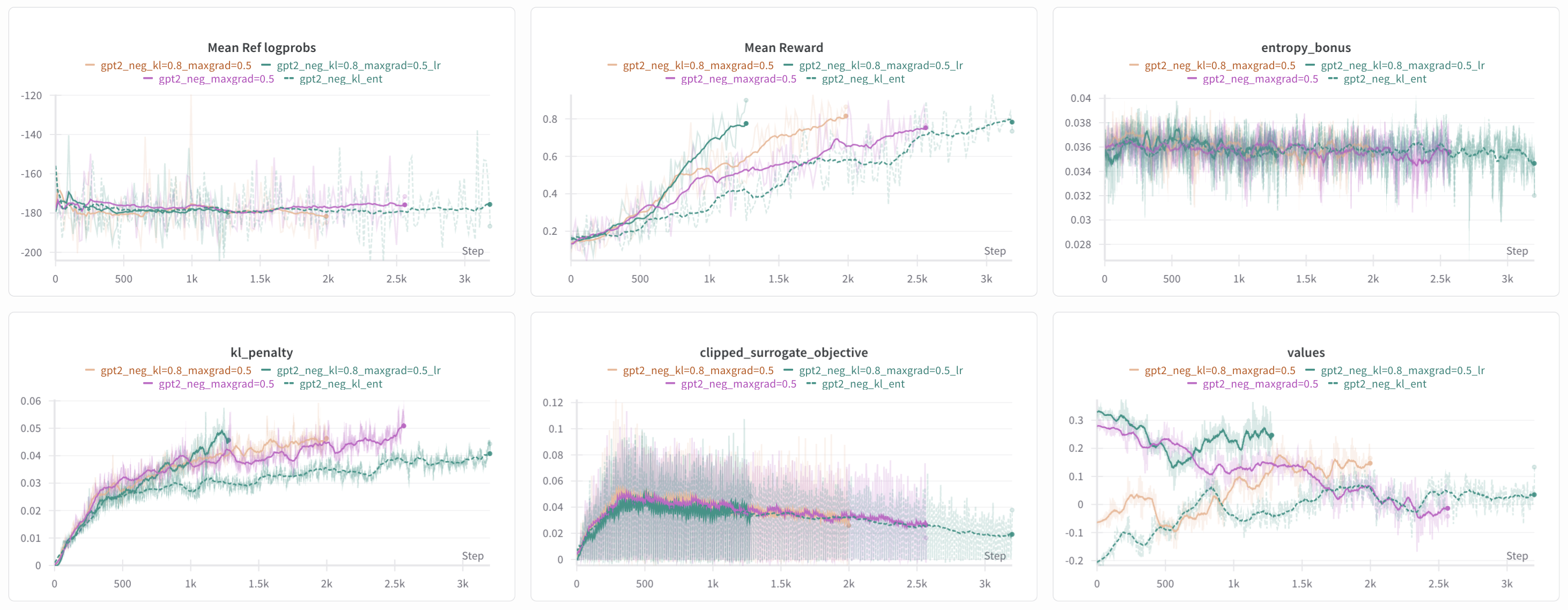 Figure 11: Log of 4 experiments with just
 kl_ent as reference. Same running average parameters apply. The gpt2_neg_kl=0.8_maxgrad=0.5_lr is the same as gpt2_neg_kl=0.8_maxgrad=0.5 but with learning rates reduced by 20%.
The hope with lowering max_grad_norm = 1.0 to 0.5 (see #11 in the “13 core implementation details” here) was to better stabilize parameter changes and prevent reward overoptimization via smaller steps. Surprisingly, decreasing max_grad_norm increased kl_penalty, though it could be explained by the small yet consistently oriented gradient updates accumulating in larger KL divergence than large yet inconsistent gradient updates.
Also, across the same early stopping parameters, decreasing max_grad_norm and kl_coef (this was already observed previously) lead to early stopping. In the same vien, decreasing the learning rates speed up reward learning, indicating that previous learning rates were pushing PPO beyond the clipping regions, so progress towards the reward was inefficient.
Indeed, the average responses seem more natural:
| Model | Reward | Sample |
|---|---|---|
| kl=0.8_maxgrad=0.5_lr | 0.9658 | This movie was really bad because the plot was a little convoluted, which I understand because I didn’t enjoy it, but I’m a little disappointed that this was done so quickly. The movie doesn’t have any story at all and it just goes with its heart. If only it were a little clearer. Also, it’s a rather short movie (3 minutes if you count the extras). Overall |
| kl=0.8_maxgrad=0.5_lr | 0.9961 | This movie was really awful and so awful that when I watched it I almost cried my eyes out with frustration. I can honestly say that, as a fan of anime, this movie was really awful. There were very few good parts on this list. Even some of this movie’s most memorable moments just weren’t memorable. It wasn’t until the end for me to find any of those parts. |
| kl=0.8_maxgrad=0.5 | 0.9966 | This movie was really bad. The music was horrible. The movie was terrible because the lyrics were so lame and the actors looked like they might die. I’m not even going to say I hated them as much as I did. I have no real idea if the characters were real. There were no signs of any emotion or remorse. It just feels like they were having some kind of bad time |
| kl=0.75_ent_clip=0.3_KLTex | 0.9927 | This movie was really bad. I mean, it’s one thing if a movie is terrible (I know that sounds horrible), and this movie is completely different. It had really poor cinematography, and it had really poor acting. And that was the only thing that really helped me. And that was that it had so much better script. It had better dialogue, better animation, better voice acting |
From this point on, max_grad_norm=0.5 and the learning rates are set as base_lr=8e-6 and head_lr=8e-5 to avoid model name elongation.
other nitty-gritty details
Now that we had a sufficient model, it might be wise to implement some details relating to PPO and RLHF (the previous global gradient clipping idea above was taken from these details!), particularly value head initialization, adapative KL control, logit/temperature scaling, and advantage whitening.
We orthogonally initalize the weights and bias of our value head, while tuning to ensure the last layer has a slightly smaller standard deviation:
def layer_init(layer: nn.Linear, std=np.sqrt(2), bias_const=0.0):
    t.nn.init.orthogonal_(layer.weight, std)
    t.nn.init.constant_(layer.bias, bias_const)
    return layer

class TransformerWithValueHead(nn.Module):
    def __init__(self, base_model):
        # other code
        self.value_head = nn.Sequential(
            layer_init(nn.Linear(d_model, 4 * d_model), std = np.sqrt(2), bias_const = 0.0),
            nn.ReLU(),
            layer_init(nn.Linear(4 * d_model, 1), std = 1.0, bias_const = 0.0)
        )

    def forward(self):
        # other code
Initializing the value head this way had very similar logs (essentially all graphs, even also ending around epoch 120) compared to the previous iteration with non-reduced learning rates, although the values seemed to converge much more quickly to 0 as opposed to 0.15 in the non-reduced model. Model responses remained coherent and negative.
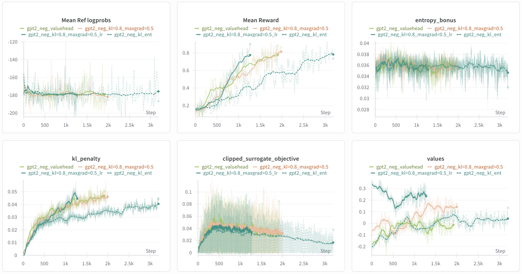 Figure 12: Log of 4 experiments with
 kl_ent other maxgrad=0.5 runs as reference. Same running average parameters apply. High reward (0.887) and high KL (0.051) were both triggered during early stopping.
Next, we test reward whitening, which we essentially have already with our normalize_reward function. We make corresponding changes in the RLHFTrainer class as well.
def whiten(values, shift_mean: bool = True, eps: float = 1e-8):
    mean = values.mean()
    var = values.var(unbiased=False)
    whitened = (values - mean) * t.rsqrt(var + eps)
    if not shift_mean:
        whitened = whitened + mean
    return whitened

def normalize_reward(reward, eps: float = 1e-8):
    # default behavior matches prior code (zero-mean, unit-variance)
    return whiten(reward, shift_mean=True, eps=eps)
However, even with the new value head, the model’s values started diverging. Since rewards keep their positive mean, the targets now propagate that positive scalar reward back through the sequence, so the value head learns positive per-token values and drifts upward. The responses also reverted back to the more formulaic and repetitive responses:
| Model | Reward | Sample |
|---|---|---|
| whiten | 0.9932 | This movie was really bad. You know what? This movie has really bad acting, and I hate actors being so bad. I hate actors playing so bad. I hate acting that they’re just terrible at making the character’s face look awful. It was actually great, though. I don’t know about you, but I have a feeling that at some point, maybe we’re going |
| whiten | 0.9932 | This movie was really pretty bad. It was really bad. I didn’t get much to say about this movie after, but I can’t imagine there was anything else out there I hated. It didn’t really make you want to see anything else. It made you think about just how bad this movie truly was, or why it made me hate the movie for so long. I love |
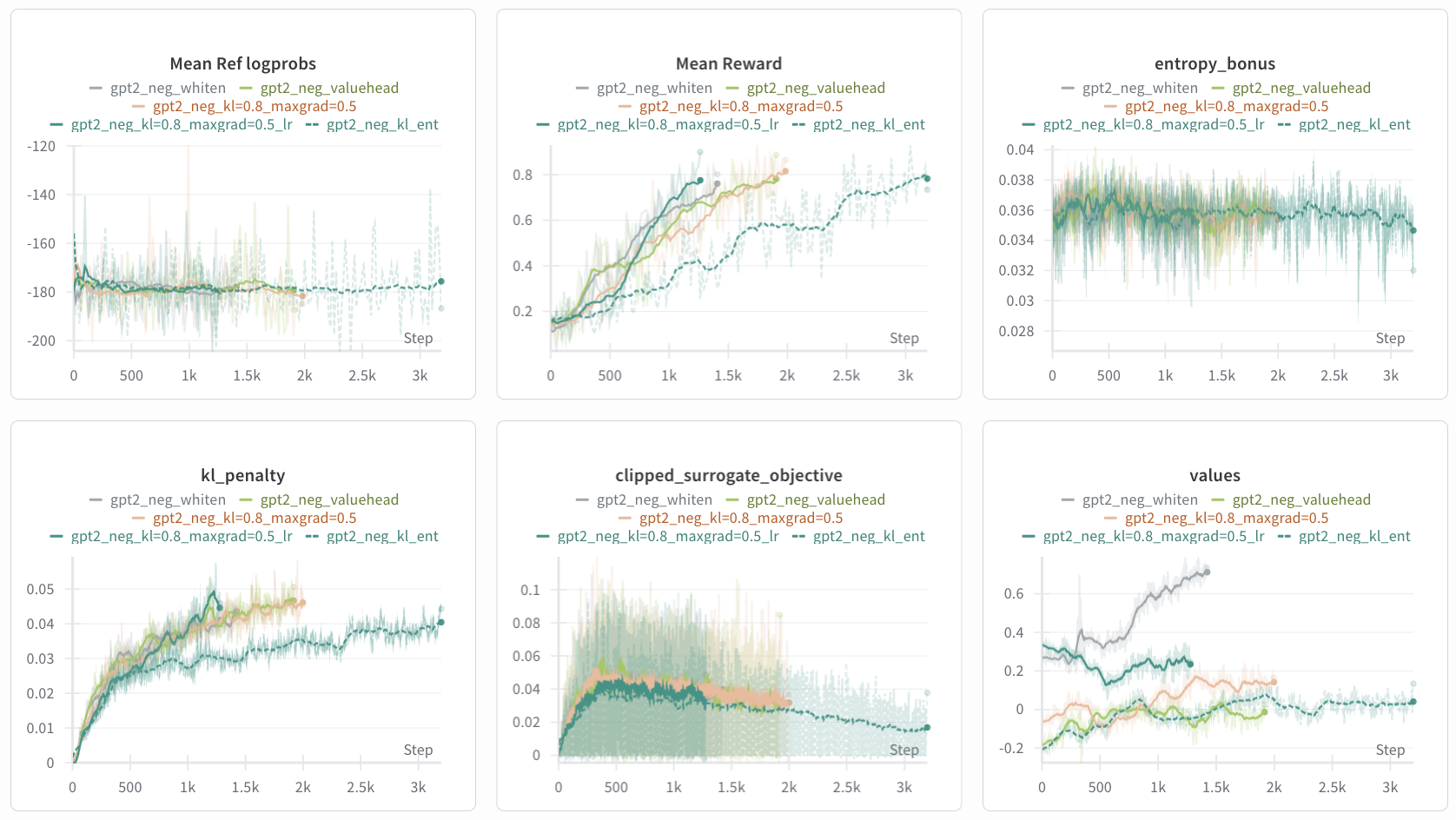 Figure 12: Log of 5 experiments with other previous runs as reference. Same running average parameters apply.
Building off of the previous analysis, we test adapative KL control and scaling logits by the inverse of the temperature. Originally, temperature = 1.0, so this has no effect on the logits. Increasing temperature, as shown previously, has diastrous effects on the coherence of the output, so we test with a lower temperature = 0.8. In the rollout phase, we change this:
scaled_logits = logits / self.args.temperature
log_probs = get_log_probs(scaled_logits, sample_ids, self.prefix_len)
For the adapative KL control, we add corresponding hyperparameters in the args while adding this:
class AdaptiveKLController:
    def __init__(self, init_kl_coef: float, target: float, horizon: int):
        self.value = init_kl_coef
        self.target = target
        self.horizon = max(1, int(horizon))

    def update(self, current_kl: float, n_steps: int, clip_coef: float) -> float:
        # proportional error scaled by clip_coef and number of steps over horizon
        proportional_error = np.clip(current_kl / max(self.target, 1e-8) - 1.0,
                                     -clip_coef, clip_coef)
        mult = 1.0 + proportional_error * (n_steps / self.horizon)
        self.value *= float(mult)
        # Keep within reasonable bounds
        self.value = float(np.clip(self.value, 1e-4, 10.0))
        return self.value

class RLHFTrainer:
    def __init__(self, ...):
        # previous code
        self.kl_controller = None
        if self.args.adaptive_kl:
            self.kl_controller = AdaptiveKLController(
                init_kl_coef=self.args.kl_coef,
                target=self.args.kl_target,
                horizon=self.args.kl_horizon,
            )

    def compute_rlhf_objective(self, minibatch):
        # previous code
        current_kl_coef = self.kl_controller.value if self.kl_controller is not None else self.args.kl_coef
        raw_kl = calc_kl_mean(logits[:, gen_len_slice], minibatch.ref_logits[:, gen_len_slice])
        kl_penalty = current_kl_coef * raw_kl

    def learning_phase(self, memory):
        # previous code
        if self.kl_controller is not None:
                new_kl = self.kl_controller.update(
                    current_kl=self.current_metrics['kl_raw'],
                    n_steps=1,
                    clip_coef=self.args.clip_coef)
                self.args.kl_coef = new_kl
Although not shown here, we seperate the calculation of the KL mean into its own function, then multiply by the coefficient in a seperate function.
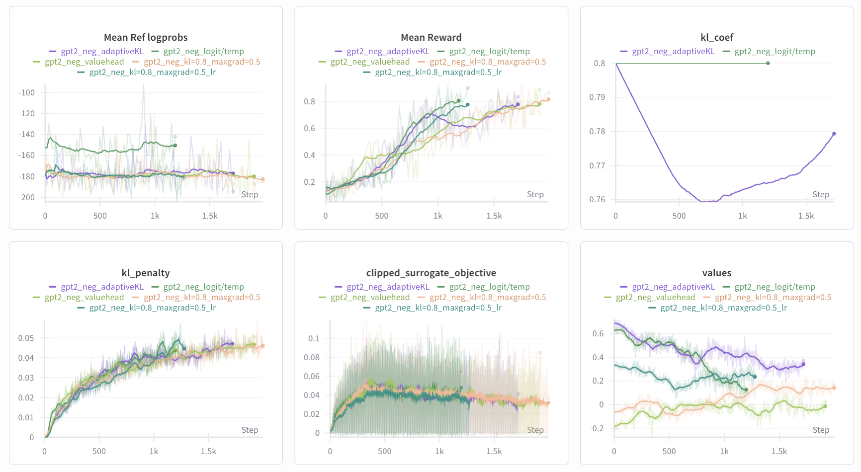 Figure 12: Log of 5 experiments with other previous runs as reference. Same running average parameters apply. The
 entropy_bonus graph has been replaced with a kl_coef graph.
Most interesting, the mean reward saw a dip in mean reward from phase 61 (step 976) to 79 (step 1264), while the kl_coef was interesting back from its minimum of 0.76 in phase 46. And accounting for the running average, the dip in the mean reward also corresponds with a roughly 0.07 increase in the values.
Sampling some of the responses from the reward dipping phase, we see that most of the negative sentiment responses are exactly as we expect them, but the frequency of positive sentiment responses began to dominant; some responses that started out negatively switched to positive sentiment after the first one or two sentences.
Looking at some responses from phase 79 (mean reward 0.4922):
| Model | Reward | Sample |
|---|---|---|
| adaptiveKL | 0.4998 | This movie was really awful! A couple of times you get an idea of the quality of the actors. This movie has the best scenes where they are not allowed to be around, but I have never seen this one. This is definitely an amazing movie. I would have never expected this movie to get it so bad. I don’t know that there are any reviews that said this was great |
| adaptiveKL | 0.1635 | This movie was really pretty, and pretty good, in its presentation, and in the script that I gave it. I thought it looked pretty good. Also, if there can be any other thing that’s really bad in terms of pacing, it should be something like the opening credits. There’s not really much going on. I think the first film was really short, but it didn’t really |
| adaptiveKL | 0.0124 | This movie was really a blast to see. I really appreciate the quality of the movie. If you’re a fan of the show and want to enjoy this movie, you can probably recommend it if you’re into geeky stuff, or something else entirely, and I don’t want to spoil any of that…but you can also get some great movies like this one. If the first one is |
The responses from the decreased but scaled temperature run was as expected but non-interesting; shorter sentences with a less rich vocabulary. Based off of the gpt2_neg_valuehead and gpt2_neg_adaptiveKL model (the latter of which is still derived from the former), we ran some final experiments playing around with the early stopping mechanism to allow it to run longer, but no significant changes were observed in the responses, although the kl_coef changed sizably (difference: 0.06) between models with temp=1.0 and temp=1.1.
results
A series of hyperparameter changes were made (across some 50+ runs). Let’s visualize the changes (or unchanged) and why.
| Variable / Change | Original Value | New Value(s) | Effect on Results |
|---|---|---|---|
| Adaptive KL controller | fixed kl_coef | enabled adaptive controller | better KL control but not a full fix |
| KL coefficient | 1.0 | 0.8 | less formulatic outputs; however KL penalty increased and some runs still early-stopped |
Entropy coefficient (ent_coef) | 0.002 | 0.01 | slightly more exploration and modest reward improvements |
Clipping coefficient (clip_coef) | 0.2 | 0.3 | increasing to 0.3 improved learning speed/stability |
Max grad norm (max_grad_norm) | 1.0 | 0.5 | smaller steps stabilized updates and improved perceived naturalness |
| Learning rates | base: 1e-5, head: 1e-4 | base: 8e-6, head: 8e-5 | more stable progress within clipping region; sped up effective reward learning compared to larger LRs |
| Prefix prompt | ”This movie was really" | "This movie was really” | removing “really” hindered training; flatter reward curves |
| Generation temperature (sampling) | 1.0 | 1.0 | Higher temp degraded coherence and quality; lower temp leads to formulaic responses |
| Logit scaling by temperature | none | logit/temperature | modest stabilization but limited impact on reward hacking. |
| Value head initialization + detached | default init | orthogonal init; smaller std on final layer | values converged to ~0 faster and more stably |
| Reward whitening / normalization | implicit normalization | explicit whitening to zero-mean/unit-variance | values drifted upward in later runs and generations became more formulaic/repetitive |
| Early stopping policy | None | adjusted thresholds | allowed longer training while preventing over-optimization risk. |
future ideas
The model is still quite stupid. The text isn’t quite coherent like any IMDb reviews you’d read online, and the consistency of negative sentiment responses isn’t there yet. That said, there are a few directions that I’m excited about:
- Multi-objective reward: combine DistilBERT sentiment with coherence, diversity (n-gram + embedding-similarity penalties via SimCSE/SBERT), and discourse consistency. Gave this a go but it wasn’t learning; rewards were stuck around where they started at 0.15-0.2. Also tried with GAE and a more uniform, non-sparse reward but that didn’t work particularly well.
- Optimization alternatives: augment Adaptive KL with per-token KL, and benchmark against DPO/IPO (RL-free preference training) with reward-ranked pairs.
- Interpretability: analyze attention heads and MLP features that activate for negative sentiment (e.g., logit lens and differences). Compare base vs RLHF heads to quantify how steering/prefix tokens shift attribution. There’s some boilerplate code in
rlhf_interp.ipynb, but I’ll need to redo the analysis soon. - Check out this paper, which does a pretty comprehensive sweep over major tricks/traps for designing an RL4LLM model. The task is LLM reasoning, but there are definitely a few parallels that can be drawn.