hunting for headroom on modded-nanoGPT (WR #82)
Modded-nanoGPT speedrunning is a popular benchmark that asks how fast 8xH100s can drive a 124M-parameter model to 3.28 validation loss on FineWeb. After iterating on dozens of failed experiments (mainly algorithmic including optimizers, activations, schedules), we propose a learnable per-(layer, head) $\tanh(\alpha)$ gate on Exclusive Self-Attention, broadened across all non-paired attention layers, which funds a 30-step schedule cut and brings the record down to 81.2 s (-0.6 s). Our submission PR is here.
This blog is taken from work done jointly with two classmates, Andrew Xu and Ben Xu, as a part of Yale’s Building AI Infrastructure class taught by Richard Yang. Thank you additionally to Richard Yang and Ryan Yang-Liu for provisioning GPUs and providing guidance throughput as well as Keller Jordan for validating and stewarding the speedrun on Prime Intellect.
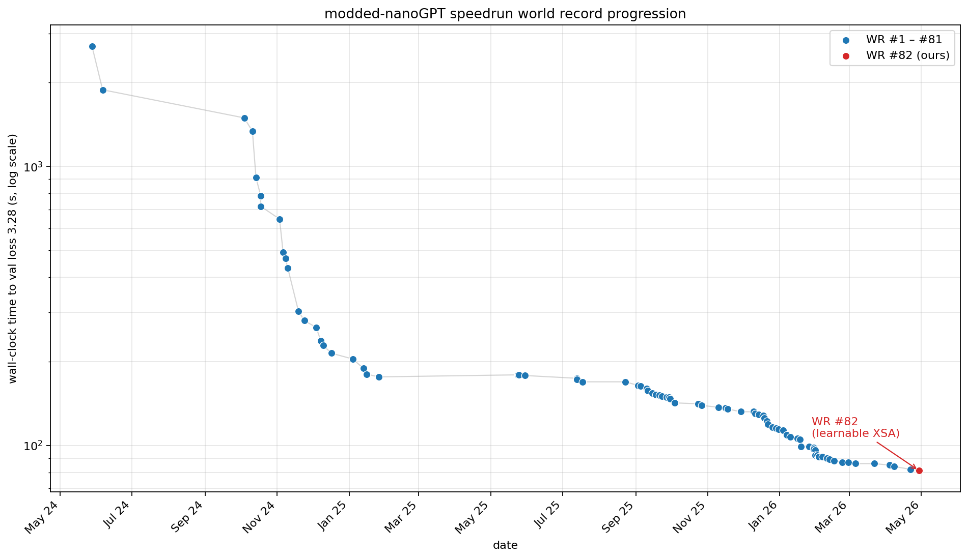 Figure 1: World-record progression of the modded-nanoGPT speedrun, May 2024 → May 2026 (log y-axis).
tl;dr
- We worked across a couple dozen branches spanning optimizer (e.g. AdaMuon), attention (e.g. selective attention), activation (e.g. Dynamic Tanh), schedule (e.g. sequence-length curriculum), and architectural changes (e.g. manifold-constrained hyper-connections). Most regressed, but some made it to clean ablations.
- We first tried the textbook deterministic version of Exclusive Self-Attention (XSA) , but every seed sat just over the 3.28 bar. Re-engineered into a learnable per-(layer, head) $\tanh(\alpha)$ gate, XSA applied across all non-paired attention layers works by letting each head learn its own correction.
- This corresponded to a 30-step cut from 1440 to 1410. Wall-clock drops by 0.554 s on 8×H200 and 0.685 s on 8×H100, comfortably under the 3.28 bar (Welch $p \approx 0.0014, n=10$).
setup
The pre-XSA record on sat around 81.8 s, the product of 81 records and nearly two years of community contributions; some ideas you might recognize are muon, FP8 lm_head, paired-head attention, value embeddings, sliding-window attention, ReLU² MLPs, and YaRN. We did most of our development on an 8×H200 box, where the same master code runs at 80.40 ± 0.11 s at val loss 3.27941 ± 0.00145 (n=10), and later re-validated on an 8×H100 box from RunPod (not offical).
| Configuration | n | Steps | Wall (s) | Δ wall | Val loss |
|---|---|---|---|---|---|
| master @ 1440 (baseline) | 10 | 1440 | 80.400 ± 0.105 | — | 3.27941 ± 0.00145 |
| master @ 1410 (naïve) | 10 | 1410 | 78.760 ± 0.046 | −1.640 | 3.28316 ± 0.00093 (fails) |
Every experiment was framed as a fixed-target optimization problem: either give back enough loss headroom to spend on a shorter schedule, or cut milliseconds per step without raising loss. We primarily focused on architecture changes, although we dabbled a bit in systems related work.
methodology
Ideas came from a few places: recent arxiv literature, deep-research sessions with frontier LLMs (Opus 4.7, GPT-5.5), and OpenAI’s parameter-golf leaderboard, where XSA itself appears among the techniques that scored well. While not fully autoresearch, there were elements of it that made this feel full-circle, especially since Andrej Karpathy, (who originated nanoGPT) has been running his own autoresearch loops to iterate on nanochat training.
Each experiment got its own branch forked off of master and typically went through two gates:
- Screen (n=1): about a third of ideas die here since the experiment introduces a clear regression (e.g. dyt diverged to NaN at every initialization we tried; hourglass-ffn was 15 % faster but +0.04 nats over the bar; xielu was almost 10 % slower wall-clock even after three kernel iterations).
- Post-Screen (n=8): this is where most ablations lived. The master noise floor at n=8 sits at $\sigma \approx 0.0014$ nats on val loss, so anything with mean effect smaller than $\approx 1 \sigma$ is below detection threshold, enough to kill bad ideas confidently.
The other invariant we held was bit-identical at step 0. Every architectural change had to begin from a configuration where the forward pass at step 0 was numerically identical to master. Usually this meant zero-initialization of any new gate or scalar (e.g. $\tanh(0)=0$ or $\sigma(\infty)=0$). The reason this matters, in retrospect, is that several branches we made fixes on top of (AdaMuon, schedule-free Adam, long-window GQA, selective attention, FoX) had bugs in their initial scaffolds that made it difficult to know whether a step-0 loss delta is a real signal.
what didn’t work
It’s probably more helpful to group the failures into patterns formed than go through all of the dead branches; not all experiments run are listed here, however.
optimizers
- AdEMAMix, AdaMuon, schedule-free Adam, Dion
- All of these add slow state (a slow EMA, a per-coordinate variance buffer, a Polyak average) that needs more than 1500 steps to warm up. AdEMAMix’s slow EMA at β₃ ≈ 0.9999 has effective horizon in the tens of thousands of steps. Perhaps these changes could actually lead to a record on the medium track, but GPT2 small to 3.28 val is probably too short and too optimized of a task.
schedule/curriculum
- Power-law decay, sequence-length curriculum, schedule-free averaging, LAWA weight-averaging, decoupled Adam/Muon LR floors
- The 3.28 bar is set almost entirely by the last 200 steps of training, where both schedules become very similar in shape but where the master’s choice has been hand-tuned. Anything that reshaped the cooldown ended up flat-to-negative because the new shape was untuned, and we run the ablations to re-tune it from scratch.
- The sequence-length curriculum is the most instructive failure here: the $L^2$-attention math says it should give you ~3 s back at the context length, and the per-step gains were real. However, each stage transition triggered a fresh
torch.compiletrace. With three stages we paid the compile tax three times, and the cumulative recompile cost was larger than the gains. The val loss $\sigma$ also bumped from 0.0014 to 0.0023, possibly the abrupt window changes were destabilizing end-of-training or the fact taht we didn’t do nearly enough runs here.
attention temperatures
- Per-(layer, head) post-QK-norm gain, SSMax log-context scaling
- We gave the optimizer learnable attention temperatures and it pushed every head back to ~1.0 within 200 steps. The existing recipe (YaRN’s per-position scaling, the global
attn_scale = 0.1) was already covering the temperature freedom we expected to find, so optimizing wouldn’t have yeilded large, significant gains. The same shape happened with attention sinks: the BOS token under the existing alignment recipe was already serving as the “attend nowhere” slot, so adding an explicit sink doubled up with no net effect.
compression
- Long-window GQA, parameter-free selective attention, register tokens (inspired by vision transformers).
- Each of these touched tensor shapes downstream of
torch.compile, which means new kernel traces. Even when the loss came back flat (or nearly so), the wall-clock regression from the compile cost erased the win. Selective attention is probably the cleanest case: the materialized(T, T)attention path is fundamentally slow on a sequence length this long.
architecture
- Dynamic Tanh, xIELU, narrower FFN (2d instead of 4d)
- Dynamic Tanh (in place of RMSNorm) diverged to NaN at every α-init, xIELU (in place of $\text{RELU}^2$) slowed down due to requiring exponents and therefore a slower kernel. An MLP intermediate layer half the size was ~13 s faster, but +0.04 nats over the bar due to loss of expression.
the one that worked: XSA
XSA (Zhai) starts from the observation that when the output y of a self-attention layer is added back into the residual stream, it includes a component aligned with the current token’s own value vector v. That’s literally what was projected from the token’s own embedding, and the residual stream already has this information. Therefore, re-injecting the self-aligned component is information-free:
XSA adds information (a per-token, post-attention correction to the residual stream) without paying any of the costs that killed everything else. Every component of the existing recipe stays in place; we just append two element-wise ops to the attention output and let the optimizer decide what to do with them. Importantly, this doesn’t involve a new matmul, a new tensor shape, a compile-time recompile, and a kernel-bandwidth penalty.
first attempt: deterministic, on layers {7, 8, 10}
Based on the paper, hardcoded, unconditional XSA on the three deepest non-paired attention layers sounds most appealing, where we hypothesized the self-attention bias would dominate. (Paired layers reshape v across head pairs in a way that doesn’t line up with XSA’s per-head subtraction, and layer 6 is MLP-only.) Twelve lines of code:
if attn_args.xsa and not self.paired:
    vn = F.normalize(v.view(B, T, self.num_heads, self.head_dim), dim=-1, eps=1e-4)
    y = y - (y * vn).sum(-1, keepdim=True) * vn
This landed at val 3.28155 ± 0.00086, wall 81.10 ± 0.38 s, a small wall improvement but every seed still sat just over the 3.28 bar. The fixed magnitude of 1.0 is the obvious thing to blame. If XSA is a “free” correction, then the optimal strength per (layer, head) is unlikely to be exactly 1.0 everywhere. Some heads might already be doing partial self-projection-removal upstream and want a small correction; others might want the full thing. This averaging isn’t optimal for everyone, so we need was a learnable per-(layer, head) gate.
second attempt: a gate
Replace the unconditional subtraction with a learnable per-(layer, head) scalar:
$$ y \leftarrow y - \tanh(\alpha_{\ell, h}) \cdot \langle y, \hat{v} \rangle\, \hat{v}, \qquad \alpha \in \mathbb{R}^{L \times H}, \quad \alpha \equiv 0 \text{ at init} $$Three things changed simultaneously:
- $\tanh$ parameterization. The actual learnable aparameter is
xsa_alphas: Parameter(num_layers, num_heads), zero-initialized. The applied strength is $\tanh(\alpha) \in [-1,-1]$ for stability, and exactly zero at init for bit-identicalness. - Adam, not Muon. The gate parameter sits in the same Adam bank as the other scalar parameters (
x0_lambdas,bigram_lambdas), withlr_mul=1.0, wd_mul=0.0. We wanted the gate to be free to settle anywhere in(−1, +1)without weight decay nudging it toward zero. - Layer set still
{7, 8, 10}. Only 18 new scalars at this point. The point was to isolate the gate as the variable, not also broaden the layer set.
if attn_args.xsa_alpha is not None and not self.paired:
    vn = F.normalize(v, dim=-1, eps=1e-4)
    proj = (y * vn).sum(-1, keepdim=True)
    alpha = torch.tanh(attn_args.xsa_alpha).type_as(y).view(1, 1, self.num_heads, 1)
    y = y - alpha * proj * vn
At n=10, this gave us a small but real loss improvement. Not enough headroom yet to fund a 30-step cut, but the direction of the result was unambiguous, and that was the first time we’d had a clean loss-positive result in the whole project.
fixing the gate
We logged the final $\tanh(\alpha_{\ell, h}$ per (layer, head) at end-of-training. A representative run:
| Layer | $\tanh(\alpha)$ per head $h \in \{0, \cdots, 5\}$ | Note |
|---|---|---|
| 7 | +0.876, +0.769, +0.837, +0.918, +0.961, +0.795 | saturated near +1 |
| 8 | +0.469, +0.084, +0.171, +0.562, +0.408, +0.379 | mid-range, head-heterogeneous |
| 10 | +0.384, +0.443, +0.635, +0.492, +0.396, +0.622 | mid-range |
Max $\alpha$ was 0.961 and mean 0.567. all 18 (layer, head) pairs were “active” ($\tanh(\alpha) > 0.05$), and it wasn’t pushing it back to 1.0 everywhere. It was pushing each head to a different value, with layer 7 saturating, layer 8 spreading across the range, and layer 10 sitting comfortably in the mid-region.
This was the strongest single signal we had in the whole project that XSA was actually doing something. The most comparable experiment was exp/qk-gain, where we added a learnable per-(layer, head) attention temperature but the optimizer converged everything to ~1.0 within 200 steps. Here, however, every head wanted a different correction strength which the gate permitted.
Layer 8’s heads had the smallest $\alpha$, so a natural next move was to drop layer 8 from the XSA set entirely to have a smaller layer set $\implies$ fewer parameters $\implies$ fewer FLOPs. However, it yielded no improvement, and what this means is that a small $\alpha$ does not imply it not being used. For example, A 0.1 gate on a long-tail correction can still be correct in a bandwidth-bound operation where the correction itself is essentially free. Thankfully, this ablation is stopped us. I don’t have a clean way to recover this lesson except in retrospect; it’s the kind of thing you only learn from running the ablation you assumed would be a free simplification.
broadening to all non-paired layers
What about the layers we hadn’t tried? We had been gating only the three deepest non-paired layers under the hypothesis that self-attention bias dominates in late layers. The diagnostic table didn’t really support that: layer 7 saturated near 1, but layers 8 and 10 were mid-range. There was no obvious pattern that said “deep layers benefit more.” So we extended XSA to all non-paired attention layers: {1, 3, 4, 7, 8, 10} for a total of 36 scalar parameters. Finally, at n=10, this gave us enough loss headroom to support the 30-step cut. Pre-step-cut val loss came in around 3.275, well below master’s 3.27941, which left us about 0.0008 nats of margin against the bar after spending the headroom.
spending the headroom
So, num_scheduled_iterations changed from 1440 to 1410. The 40-step extension iter count is held fixed, so the total runtime is 1450 minus the 30 saved steps. Wall-clock dropped to 79.85 s; val loss came in at 3.27865 at n=10, comfortably under the 3.28 bar. The full ablation:
| Configuration | n | Steps | Wall (s, µ ± σ) | Δ wall | Val loss (µ ± σ) |
|---|---|---|---|---|---|
master @ 1440 (baseline) | 10 | 1440 | 80.400 ± 0.105 | — | 3.27941 ± 0.00145 |
master @ 1410 (naïve) | 10 | 1410 | 78.760 ± 0.046 | −1.640 | 3.28316 ± 0.00093 (fails) |
| Gated XSA @ 1410 (PR) | 10 | 1410 | 79.846 ± 0.206 | −0.554 | 3.27865 ± 0.00105 (passes) |
Loss improvement vs. master is −0.00076 nats (Welch $p \approx 0.0014, n=10$). The naïve step cut is faster but fails the 3.28 bar by 0.00316 nats with 4$\sigma$ confidence. On the 8×H100 box from RunPod, the same PR gives Δ wall = −0.685 s at val loss 3.27890 ± 0.00118 (n=11), vs. the WR #80 baseline at 85.902 ± 0.069 s (n=7); the differene is mostly likely attributed to differences in hardware setups between RunPod and Prime Intellect.
Only ~15 LoC (excluding comments) were changed in train_gpt.py: the gate parameter declaration, the normalize-and-subtract on FlashAttention’s output, registration in the Adam parameter bank with lr_mul=1.0, wd_mul=0.0, and the step reduction.
takeaways
The change that worked was almost embarrassingly small, and it worked because XSA augments the existing solution space rather than replacing part of it. The master branch is a tight local optimum along nearly every direction we probed, but only along the directions the existing recipe already explored, and XSA opened up a new one. Every replacement has to beat a version of the existing component that’s been hand-tuned for months by people who knew what they were doing; every augmentation only has to beat zero, and zero is what the existing system gets to use by default. The asymmetry is in your favor.
A few specific lessons I learned from getting there:
- Optimizer testing is relatively cheap and very iterable. Sorry for coming back to this again, but on
exp/qk-gain, the optimizer pushed every per-head attention temperature back to 1.0 within 200 steps; onexp/xsa-gated, it pushed each (layer, head) gate to a non-zero head-heterogeneous value with $\alpha$ up to 0.96. The first answer says the existing architecture is locally optimal in that direction; the second says it isn’t. The cost of asking is ~18-36 scalar parameters and one training run. - Small $\alpha$ doesn’t mean “not used.” Layer 8’s gates had the smallest $\alpha$ in our diagnostic, and the natural simplification was to drop layer 8 from the XSA set. Pruning didn’t help — even a 0.1 correction earns its place when the underlying op is essentially free. We almost shipped a worse PR over this.
torch.compileis can be a tax on tensor-shape changes. Five branches in this project paid compile or kernel-shape costs that erased the per-step gains they targeted. XSA slipped through partly because the gate doesn’t change any tensor shapes — it just adds two element-wise ops on existing tensors.